|
|
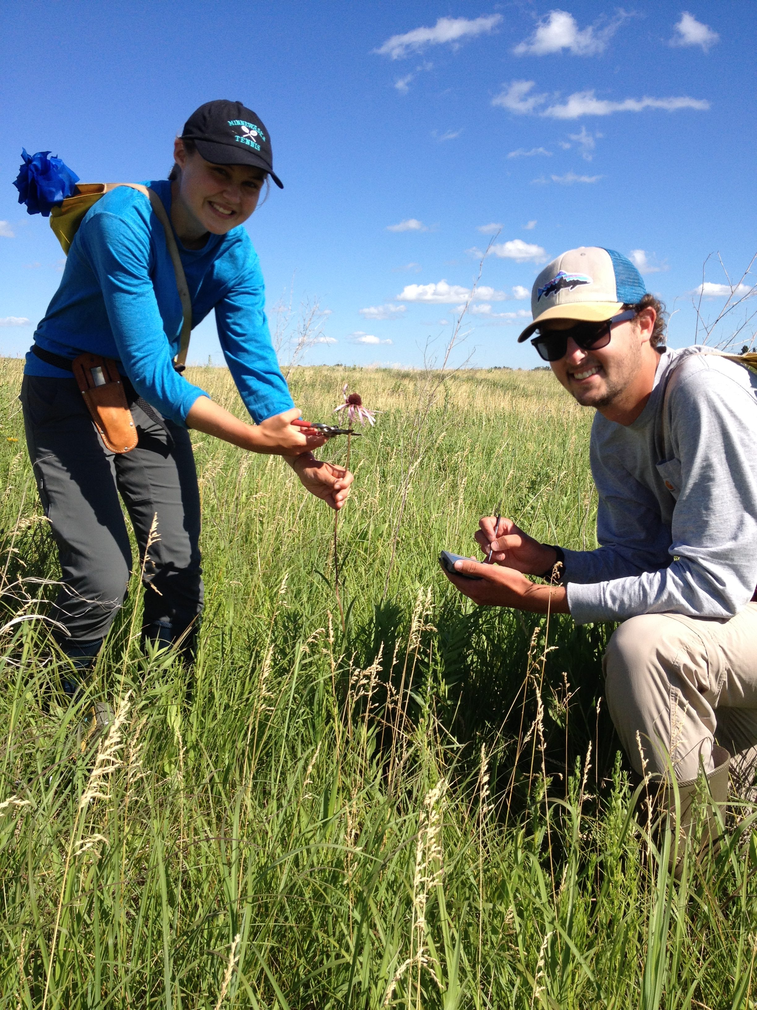
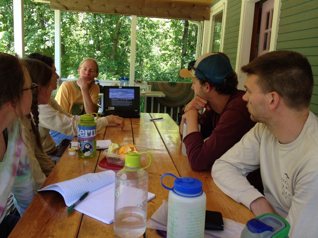
 Anna and Will decapitate a plant. It’s Echinacea pallida which is not native to Minnesota. Echinacea pallida is an Echinacea species that is not native to Minnesota. In July 2017, we identified 100 flowering E. pallida plants with 222 heads that were planted in a restoration at Hegg Lake WMA. Every year for the past several years, we have visited the E. pallida plants, taken phenology data, and chopped off their heads. On July 7, 2017 when we collected the data, the maximum male row was 19, meaning flowering started about 19 days earlier–June 18, 2017. E. angustifolia in the remnants started flowering on June 24, about a week later. 17 of the 222 E. pallida heads were still buds on 7 July, so these plants would have continued flowering for awhile.
We went back to check if we missed any heads on 31 August and found two. They were done flowering, but hadn’t dropped seeds.
Start year: 2011
Location: Hegg Lake WMA restoration
Overlaps with: Echinacea hybrids (exPt6, exPt7, exPt9), flowering phenology in remnants
Physical specimens: 222 heads were cut from E. pallida plants and likely decomposed. We brought two heads back with us to Chicago.
Data collected: A csv in ~Dropbox/remData/105_assessPhenology/phenology2017 with tag, row number the male florets were at on July 7, 2017 for each head, and initials of the data collector.
GPS points shot: We shot points for the 100 flowering E. pallida plants.
Products: In Fall 2013, Aaron and Grace, externs from Carleton College, investigated hybridization potential by analyzing the phenology and seed set of Echinacea pallida and neighboring Echinacea angustifolia that Dayvis collected in summer 2013. They wrote a report of their study.
Previous team members who have worked on this project include: Nicholas Goldsmith (2011), Shona Sanford-Long (2012), Dayvis Blasini (2013), and Cam Shorb (2014)
You can find more information about Echinacea pallida flowering phenology and links to previous flog posts regarding this experiment at the background page for the experiment.
 Marisol, our 2017 Lake Forest College intern! This fall the Echinacea Project had a Lake Forest College intern, Marisol. In Marisol’s 16-hour internship over 4 weeks, she accomplished a lot! Her primary goal was to assess if the seed counter will be useful in our ACE protocol. Currently, volunteers scan achenes and then count them with our counting software online. The seed counter could potentially remove these steps and make the process more efficient.
Marisol did a few experiments with the seed counter. She determined the best sensitivity and speed settings for counting Echinacea achenes, by running packs of achenes through the seed counter multiple times and comparing those counts to her manual counts. She found that the most accurate sensitivity and speed is 8 and 70, respectively.
Marisol also determined the types of achenes that get counted and the types of achenes that often get missed. Usually, achenes that are really small, thin, and broken don’t get counted at all. Broken achenes that are still pretty large often get counted (about 2/3 of the time). Achenes that are full and above a certain size get counted 100% of the time.
In the mini-internship class, Marisol presented her findings to her classmates. See her poster below!
 Marisol’s final poster for her mini-internship! Click to enlarge.
This year, the number of flowering plants in our main experimental plot (exPt1) dropped in half compared to last year. This might be due to the lack of a burn in the prior fall or spring. Plot 2 (exPt2) had about the same number of heads in ’16 & ’17.
In exPt1, we kept track of approximately 72 heads. The peak date was July 19th. The first head started flowering on July 2nd and the last head finished up on August 21st. In contrast, we kept track of 1076 heads in exPt2, about 140 more than last year! The peak date for these Echinacea was a bit earlier, July 13th. exPt2 heads also started and ended earlier (June 22 – August 19).
We harvested the heads at the end of the field season and brought them back to the lab, where we will count fruits (achenes) and assess seed set.
 Flowering schedules for 2017 in exPt1 and exPt2. Black dots indicate the number of flowering heads on each date. Gray horizontal line segments represent the duration of each head’s flowering and are ordered by start date. The solid vertical line indicates peak flowering, while the dashed lines indicate the dates when 25% and 75% of heads had begun flowering, respectively. Note the difference in y-axes between the two plots. Click to enlarge! Start year: 2005
Location: Experimental Plots 1 and 2
Overlaps with: Heritability of flowering time, common garden experiment, phenology in the remnants
Physical specimens: Harvested heads from both experimental plots are in the lab at CBG. The ACE protocol for these heads will begin soon.
Data collected: We visit all plants with flowering heads every 2-3 days starting before they flower until they are done flowering to record start and end dates of flowering for all heads. We managed phenology data in R and added it to our long-term dataset. The figures above were generated using package mateable in R. If you want to make figures like this one, download package mateable from CRAN!
You can find more information about phenology in experimental plots and links to previous flog posts regarding this experiment at the background page for the experiment.
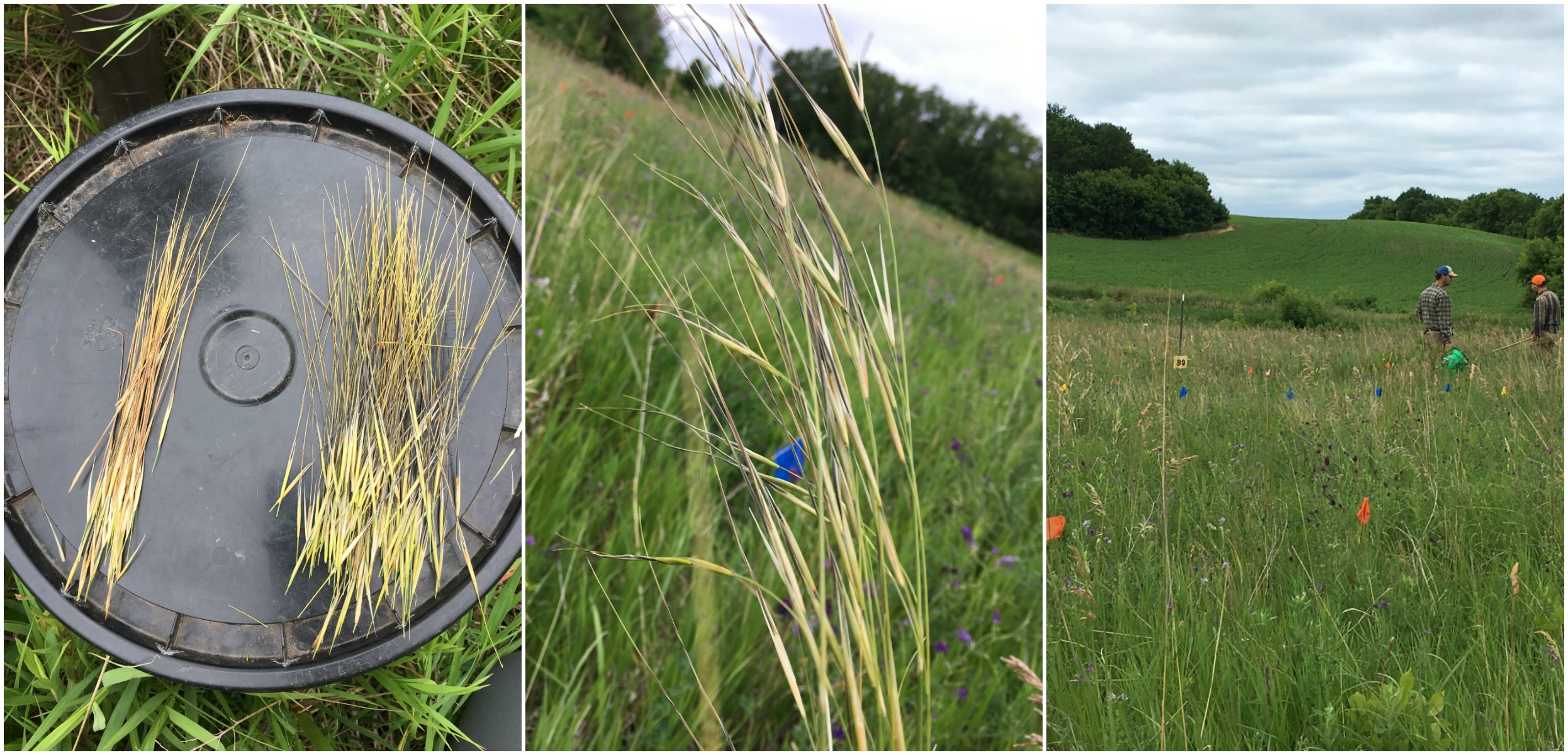
This summer we found 52 basal Stipa plants and 209 flowering plants! The flowering Stipa plants had a median of 15 fruit per plant. Our largest flowering Stipa plant had 301 fruits and 31 culms. We harvested around 5000 fruits from experimental plot 1! These Stipa plants, or porcupine grass (Hesperostipa spartea) were planted as seeds in 2009 and 2010.
 A Stipa collage created by Anna with collected fruits, a flowering plant, and Will and Wes searching for stipa. Start year: 2009
Location: Experimental plot 1
Physical specimens: Fruits from the 209 flowering plants were broadcasted in experimental plot 2.
Data collected: There are currently 3 datasets in the Stipa folder in CGData (~Dropbox/CGData/Stipa/225_measure/measure2017/)
- 20170628StipaSearchData.csv: 50 records from 28 June 2017. We searched for basal and flowering Stipa and recorded row and position, culm count, fruit count, aborted fruit count, missing fruit count, and notes.
- exPt1StipaSearch20170705.csv: 200 records from 28-29 June 2017. This csv includes rows with position 859 and status “Other (Note)”, indicating the row was searched but no stipa was found. When Stipa was found, status, row, position, culm count, fruit count, aborted fruit count, missing fruit count, and notes were recorded.
- 20171109StipaSearchData.csv: 69 records from 2 August 2017 and 9 August 2017. In this csv, predetermined rows and positions (where Stipa were found in previous years) were searched and the same information was collected as the other csvs. Since this was later in the season, all fruits had already dropped–but they could still be counted.
Products:
- Josh Drizin’s MS thesis included a section on the hygroscopicity (reaction to humidity) of Stipa awns. View his presentation or watch his short video.
- Joseph Campagna and Jamie Sauer (Lake Forest College) did a report on variation in Stipa’s physical traits within and among families in 2009
You can find out more about Stipa in the common garden and links to previous flog posts about this project on the background page for this experiment.
We had a big year for censusing plants in natural remnant populations. In 2017 we did both total demo, visiting all plants, and flowering demo, visiting just plants that flowered this year. Check out the chart below to see what we focused on at each site:
| Total Demo |
Aanenson, Around LF (partial), Common Garden, East of Town Hall, East Riley, Hegg Lake, Landfill West, Loeffler Corner East, NRRX, recruit he, recruit hp, recruit hs, Riley, RRX, South of Golf Course, Steven’s Approach, transplant plot |
| Flowering Demo |
Around LF, BTG, DOG, Elk Lake Road East, Golf Course, KJs, Krusemark, Landfill East, Liatris Hill, Loeffler Corner West, Near Town Hall, Nessman, NNWLF, North of Golf Course, NWLF, On 27, recruit el, recruit hw, recruit ke, recruit kw, RRXDC, Staffanson East Unit, Staffanson West Unit, Tower, Town Hall, West of Aanenson, Woody’s, Yellow Orchid Hill East, Yellow Orchid Hill West |
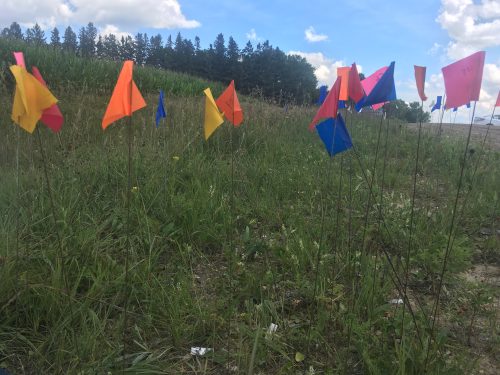
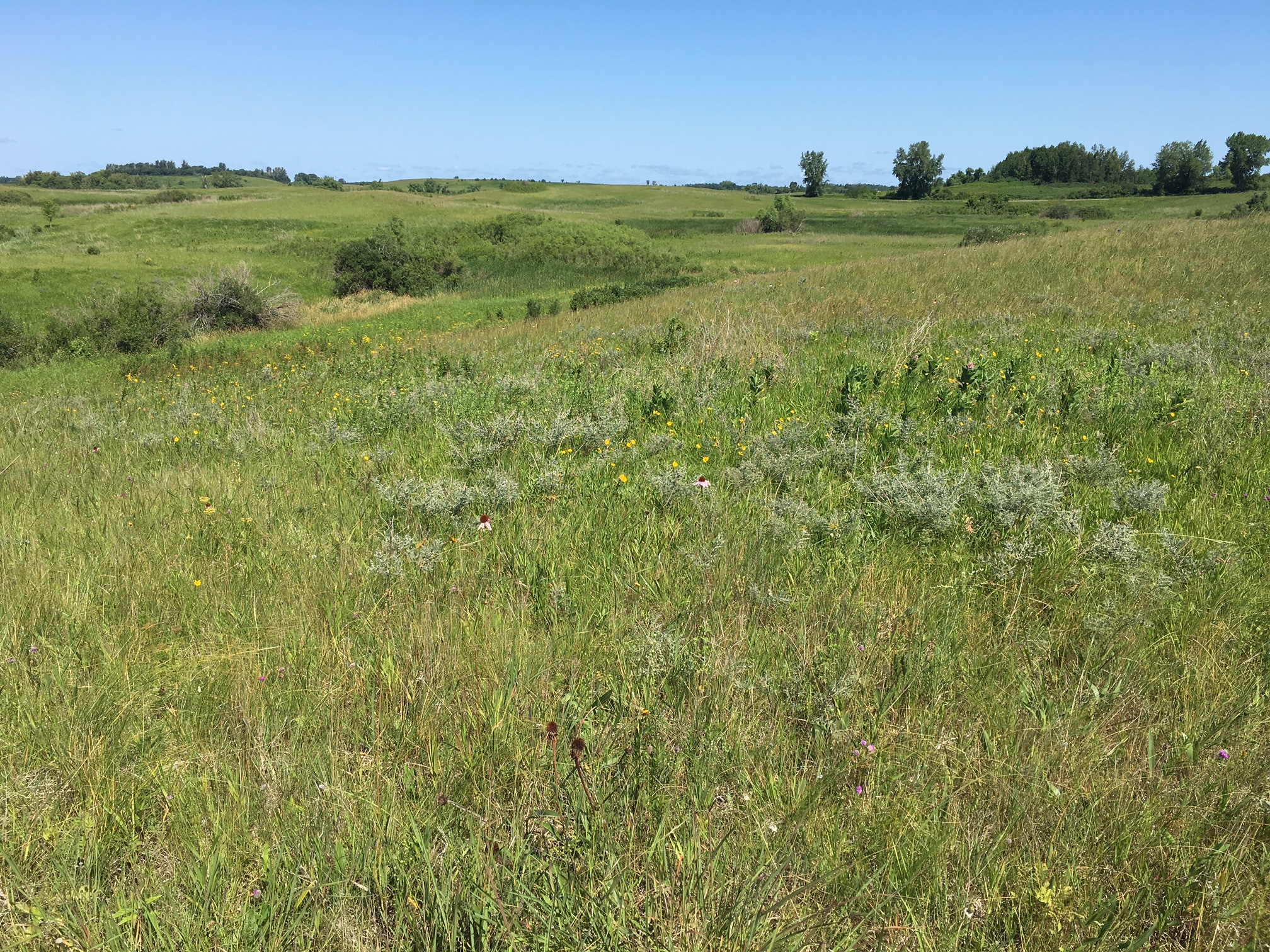
 We stake to locations where flowering plants have been found in the past and place a flag there. This is the East Riley roadside remnant, an area with a lot of Echinacea close together and a high chance of getting mowed. When we find a new flowering Echinacea plant, we give it a tag and get its location with a survey-grade GPS (better than 6 cm precision). Then, we can revisit this plant for years to come and monitor its survival and reproduction.
This season we added 5945 demo records and about 1375 survey records to our database. After over 20 years of this method, we now have a very rich longitudinal dataset of life histories including thousands of plants. REU Will Reed was a huge help organizing demo tasks for Team Echinacea over the summer and helping out with demap (the demographic census database) during the year.
Year started: 1996
Location: Roadsides, railroad rights of way, and nature preserves in and near Solem Township, Minnesota.
Overlaps with: Flowering phenology in remnants, fire and flowering at SPP
Data collected: demo records include Flowering status, number of rosettes, number of heads, neighbors within a 12 cm radius of plants found. These are all taken with PDAs that sync with an MS Access database. They are all transferred to the demap R repository in bitbucket with git version control.
GPS points shot: Points for each flowering plant this year shot mostly in SURV records, stored in surv.csv. Each location should be either associated with a loc from prior years or a point shot this year.
Products:
- Amy Dykstra’s dissertation included matrix projection modeling using demographic data
- Project “demap” merges phenological, spatial and demographic data for remnant plants
You can find out more about the demographic census in the remnants and links to previous posts regarding it on the background page for this experiment.
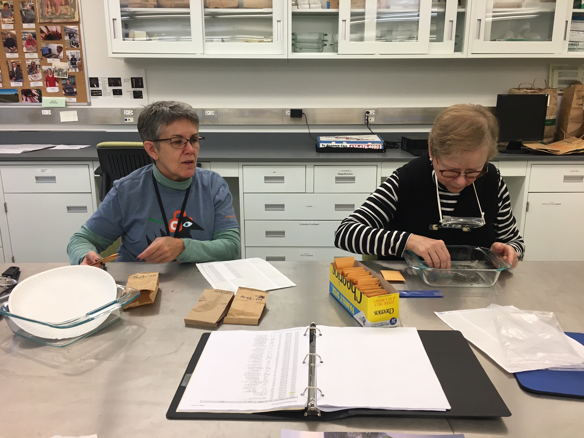
Anne and Leslie are hard at work rechecking heads that have been cleaned from 2016. This is an important job in our ACE protocol as it makes sure that no achenes are left behind before they get counted and randomized!
Anne and Leslie rechecking Echinacea heads from 2016
This summer, Amy and members of Team Echinacea continued to monitor the progress of Echinacea plants in her local adaptation plots. We found 221 basal plants, but no flowering plants this year. Amy has 3 sites: Western South Dakota, Central South Dakota, and West Central Minnesota. At each site achenes from all sites have been sowed. Team Echinacea is able to help with the assessment of survival and fitness traits of the individuals in the Minnesota plot.
 Amy presents her local adaptation research so far at lunch this summer. Start year: 2008
Location: Grand River National Grassland (Western South Dakota), Samuel H. Ordway Prairie (Central South Dakota), Staffanson Prairie Preserve (West Central Minnesota), and Hegg Lake WMA (West Central Minnesota).
Overlaps with: Dykstra’s interpopulation crosses
Data collected: Plant fitness measurements (plant status, number of rosettes, number of leaves, and length of longest leaf)
You can find more information about Amy’s local adaptation experiment and links to previous flog posts regarding this experiment at the background page for the experiment.
This summer, we found 68 basal plants in the crossing experiment. None of these plants have ever flowered, but maybe next year! We measured plant status, number of rosettes, number of leaves, and length of the longest leaf of the individuals. We also noted damage (herbivory) to the leaves.
These data will allow Amy to test how mating with individuals from other populations affects Echinacea fitness. She planted 15,491 achenes, the offspring of crosses from six of the largest remnant populations. Populations might either benefit or suffer from crossing with plants from another population.
Hegg Lake WMA Start year: 2008
Location: Hegg Lake WMA
Overlaps with: Dykstra’s local adaptation
Data collected: Plant fitness measurements (plant status, number of rosettes, number of leaves, and length of longest leaf)
Products: Read about Amy’s analysis of the interpopulation crossing experiment in her flog post.
You can find more information about Amy’s experiment and links to previous flog posts regarding this experiment at the background page for the experiment.
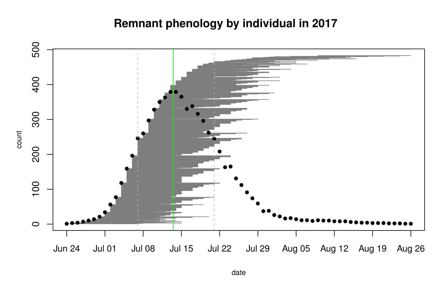
In 2017, according to our preliminary data, flowering began on June 24th with one head at the Aanenson remnant. The latest bloomer was a 5-headed plant at Steven’s Approach, and the last day its last head shed pollen was August 26th. Peak flowering for the 9 remnants we observed this year was July 13th. There was a total of 427 flowering plants producing 575 flowering heads. The figure below was generated with R package mateable, which was was developed by Team Echinacea to visualize and analyze phenology data.
 The gray shaded area is made up of horizontal gray lines, each representing the duration of one flowering head. The vertical green line represents the peak flowering date, July 13th. On average, heads flowered for approximately 2 weeks. From 2014-2016, determining flowering phenology was a major focus of the summer fieldwork, with Team Echinacea tracking phenology in all plant in all of our remnant populations. Stuart began studying phenology in remnant populations between 1996 and 1999 and several students also studied certain populations in following years. The motivation behind this study is to understand how timing of flowering affects the reproductive opportunities and fitness of individuals in natural populations.
Start year: 1996
Location: roadsides, railroad rights of way, and nature preserves in and near Solem Township, MN (2017: Aanenson, Around Landfill, East Elk Lake Road, Nessman, Northwest Landfill, Steven’s Approach, Staffanson Prairie Preserve, Town Hall)
Overlaps with: Phenology in experimental plots, demography in the remnants, reproductive fitness in remnants
Physical specimens:
- We harvested 121 Echinacea heads at 8 of the 28 remnants. These were harvested from Lea and Tracie’s “rich hood” (richness of neighborhood) plots. Not all harvested heads were monitored for the phenology dataset.
Data collected: We identify each plant with a numbered tag affixed to the base and give each head a colored twist tie, so that each head has a unique tag/twist-tie combination, or “head ID”, under which we store all phenology data. We monitor the flowering status of all flowering plants in the remnants, visiting at least once every three days (usually every two days) until all heads were done flowering to obtain start and end dates of flowering. We managed the data in the R project ‘aiisummer2017′ and will add it to the database of previous years’ remnant phenology records.
GPS points shot: We shot GPS points at all of the plants we monitored. The locations of plants this year will be aligned with previously recorded locations, and each will be given a unique identifier (‘AKA’). We will link this year’s phenology and survey records via the headID to AKA table.
You can find more information about phenology in the remnants and links to previous flog posts regarding this experiment at the background page for the experiment.
In 2017, we monitored the start and end dates of flowering for the 676 flowering plants (1116 heads) in experimental Plot 2. The first head started shedding pollen on June 26 and the latest bloomer ended flowering on August 19. Peak flowering was on July 13th. Note that these dates are subject to change as this is preliminary data that has not been fully cleaned and analyzed.
To examine the role flowering phenology plays in the reproduction of Echinacea angustifolia, Jennifer Ison planted this plot in 2006 with 3961 individuals selected for extreme (early or late) flowering timing, or phenology. Using the phenological data collected this summer, we will explore how flowering phenology influences reproductive fitness and estimate the heritability of flowering time in Echinacea angustifolia.
One of the earlier flowering plants at exP2 this summer, a plant with 5 heads at Row 2 Position 1. Start year: 2006
Location: Experimental Plot 2, Hegg Lake WMA
Overlaps with: phenology in experimental plots, phenology in the remnants
Physical specimens: We harvested approximately 1081 heads from exPt 2 (preliminary inventory). Some of these heads had a major loss of achenes, either due to the early flowering time that we were not expecting or windy and rainy weather that dispersed the achenes quickly. We brought the harvested heads back to the lab, where we will count fruits and assess seed set for each head.
Data collected: We visited all plants with flowering heads every two days (three days after weekends) until they are done flowering to record start and end dates of flowering for all heads. We will manage phenology data in R and add it to the full dataset.
Products: Will estimated heritability of flowering time using data from 2015 and presented his findings last summer at ESA (see his poster). He is continuing this work by assessing how heritability estimates differ between years in burn and non-burn years, now including 2016.
You can find more information about the heritability of flowering time and links to previous flog posts at the background page for the experiment.
|
|