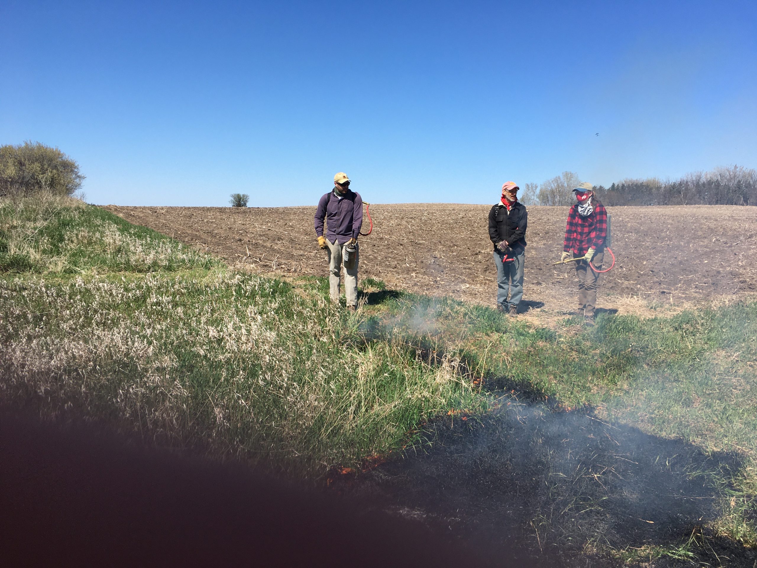
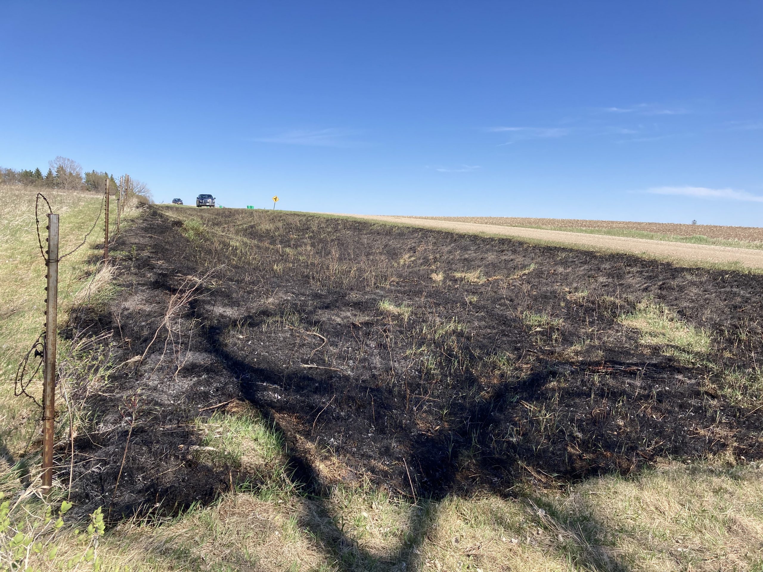
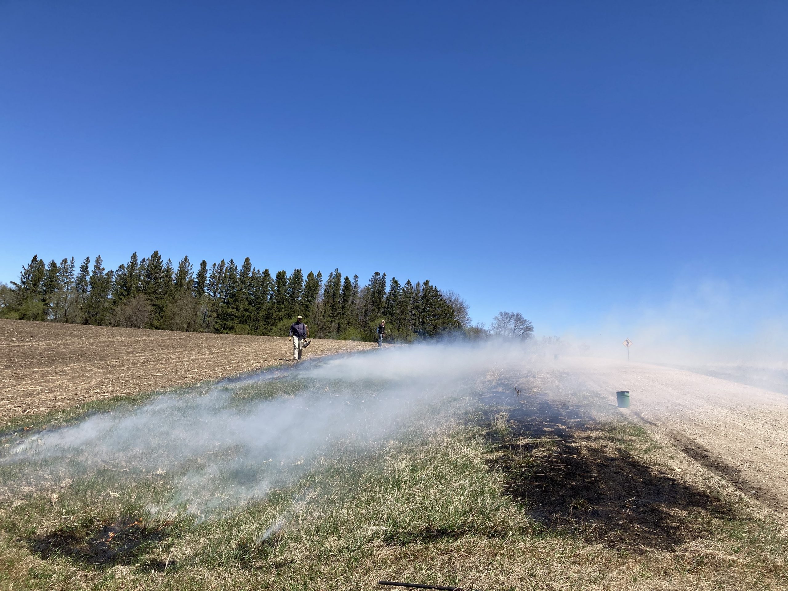
After wrapping up our first remnant burn of the season at east riley, the crew ventured into the wild western prairies of Grant County. Earlier in the day, Mia mowed burn breaks at yellow orchid hill east. This roadside patch had considerably more fuel than east riley and NW winds remained stiff when we arrived. Once water buckets had been staged and the crew briefed, we ignited a test fire in the southeast corner. This fire backed beautifully against the wind, moving steadily and burning fuel completely. One of my takeaways from burns this spring is that prescribed burns in a little lower relative humidity (RH = 25-30) and a little higher winds (12-18 mph sustained) seem to produce great results in burn units where brome is the primary fuel.
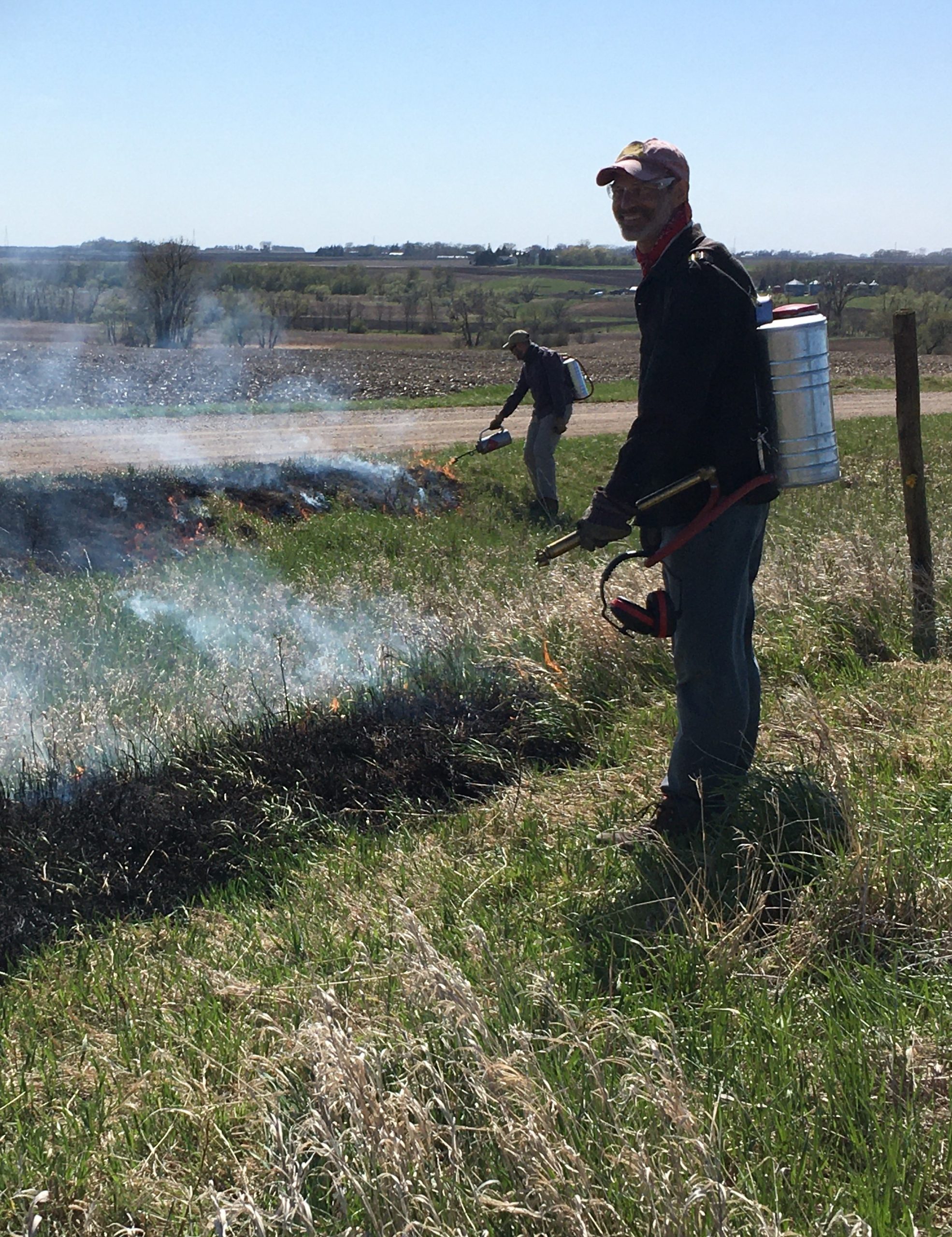
A nice sequence of photos illustrating how the burn at yoh.e progressed. We started with a test fire and observed that small fire before proceeding to burn the entire unit. We decided to ignite the downwind edge of the burn unit and allow that fire to back against the stiff wind. Looking at the fourth and fifth photos, you can see the wind push smoke to the south as the fire backs slowly against the wind moving north.
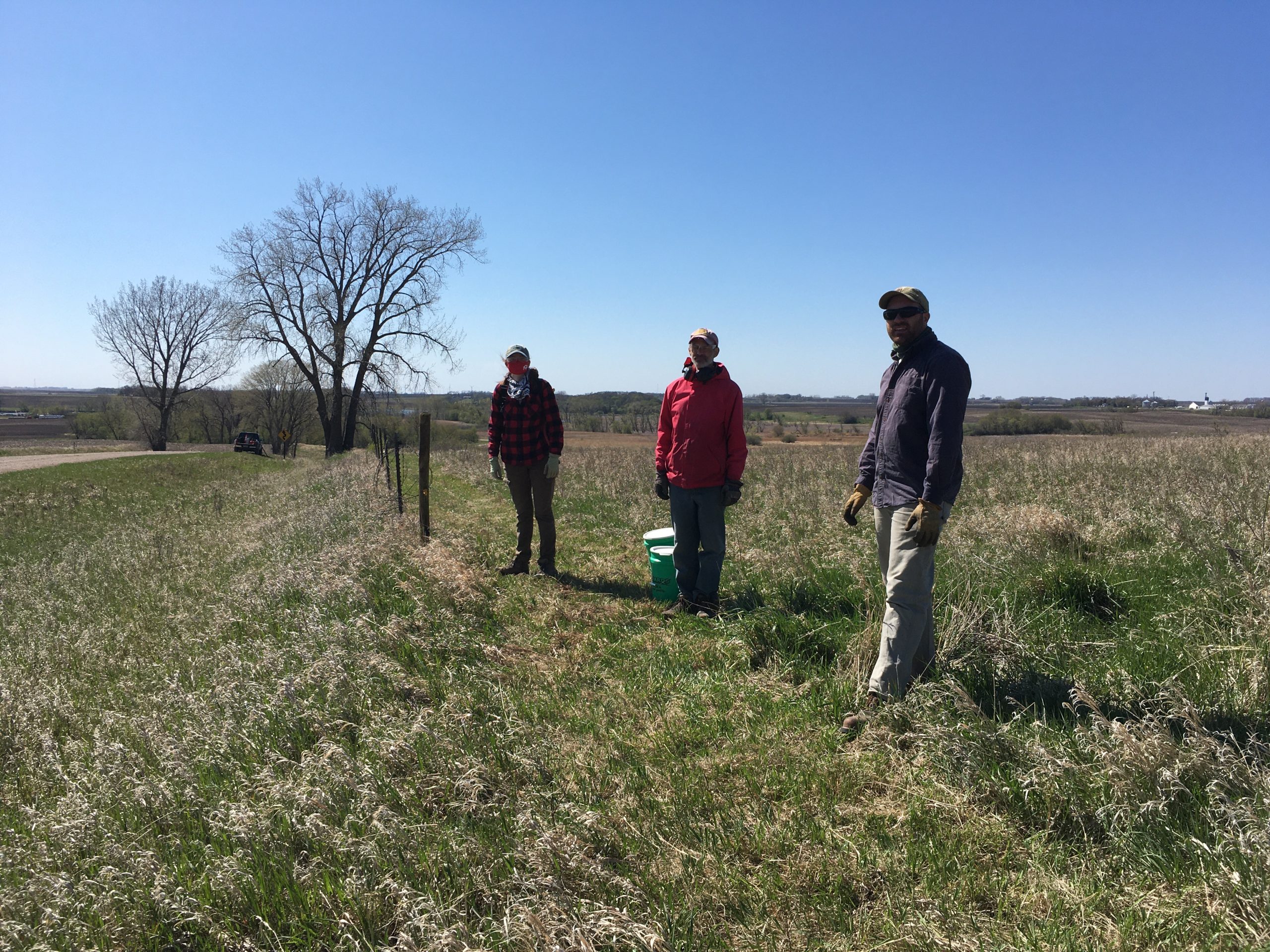
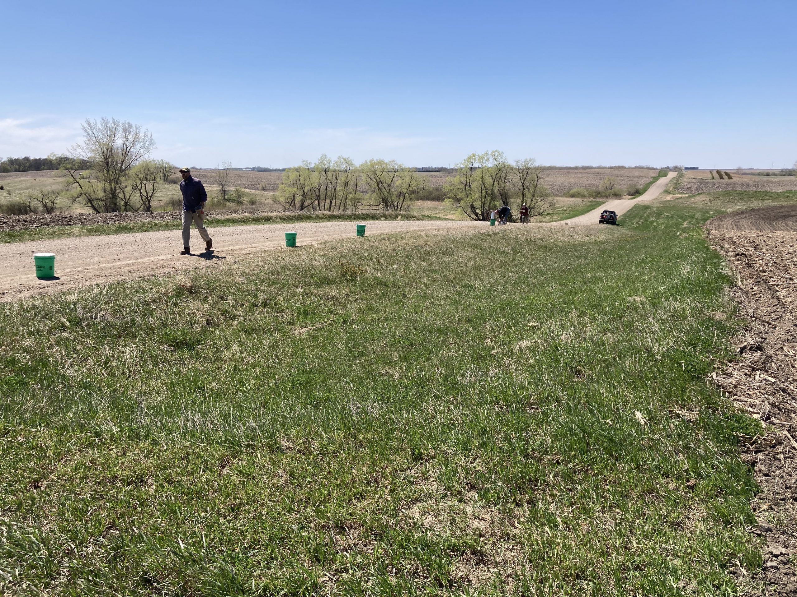
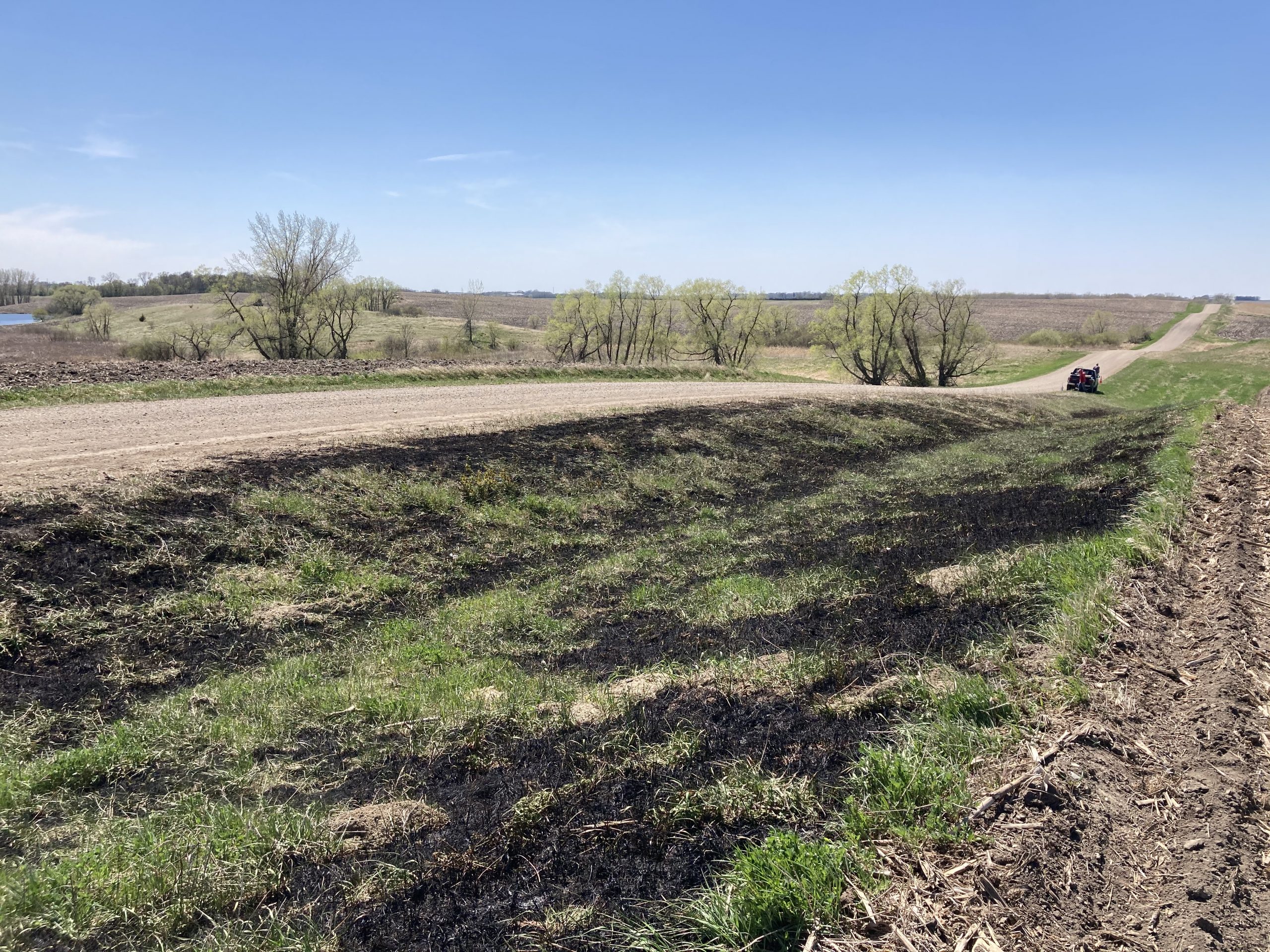
We decided to let the fire back against the wind across the entire burn unit. Once sufficient black had been established in the southeast corner of the unit, we ignited a backing fire along the entire southern edge of the unit along Wennersborg Rd. After fire lines were secured, Gretel grabbed the push power and finished mowing burn breaks at yellow orchid hill west while Jared, Stuart, and Mia extinguished any remaining hotspots. 30 minutes after ignition, we were left with an almost entirely blackened burn unit. Beautiful, predictable prescribed burn!
Temperature – 53 F Relative humidity – 30% Wind speed (max gusts) – 18 (21) mph wind direction – NNW Ignition time – 3:44 PM End time – 4:14 PM Burn crew: Jared, Stuart, Gretel, Mia
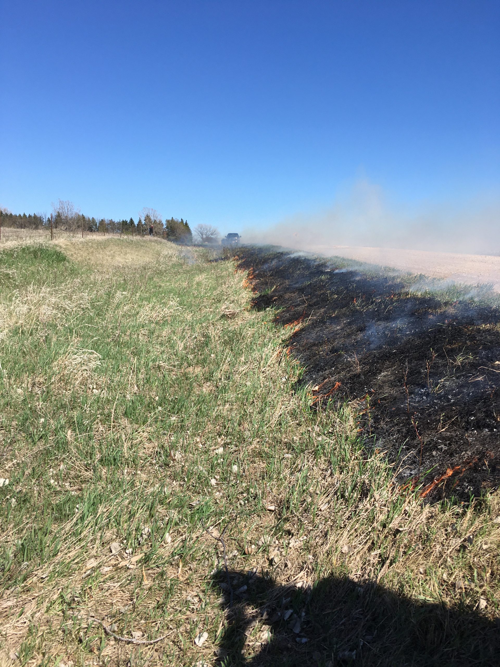
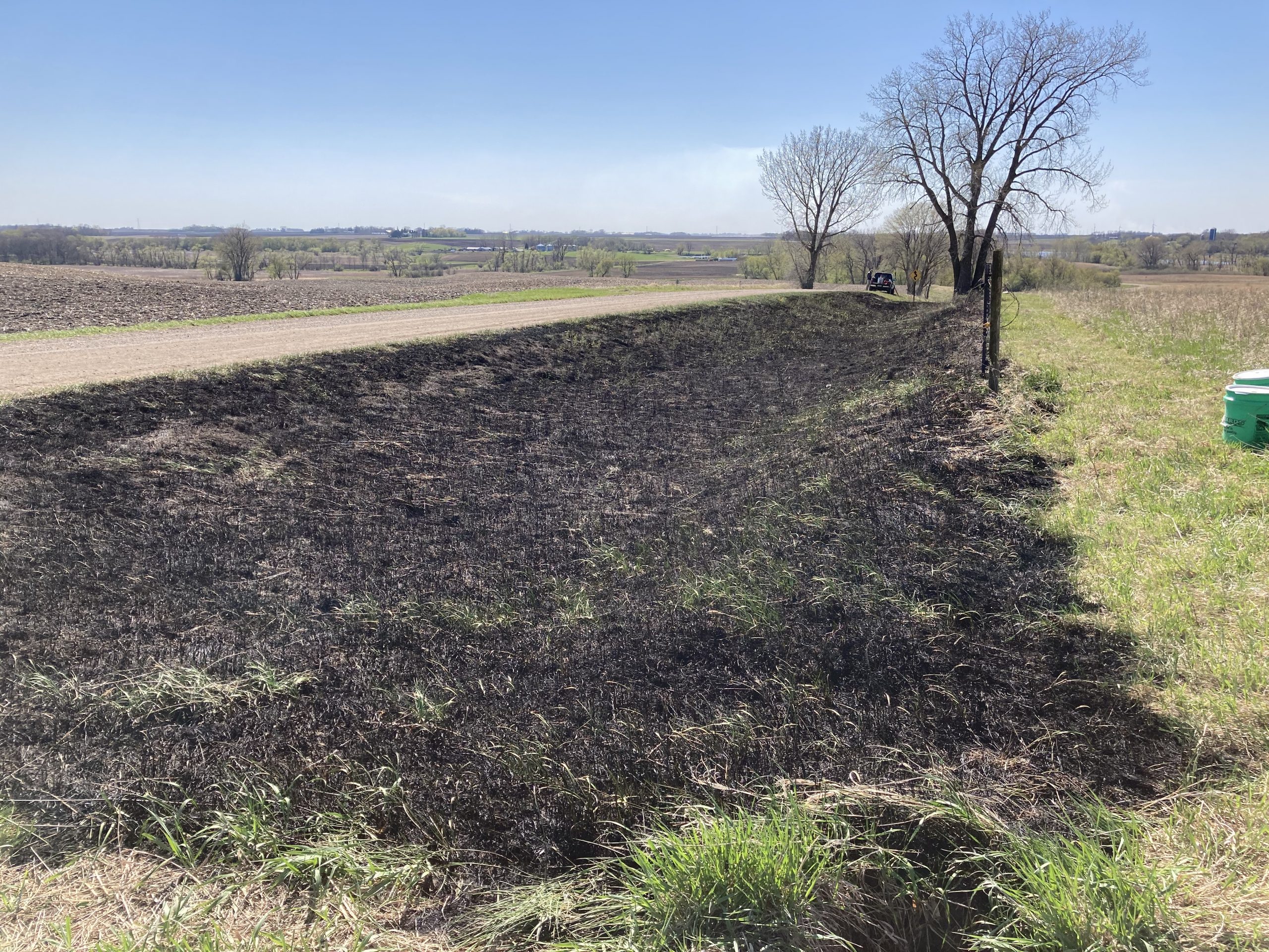
Before and after photos looking east along Wennersborg Rd
Before and after photos looking west along Wennersborg Rd
After 5 months of preparation, we officially applied the first experimental treatments for our NSF proposal to study prescribed fire effects on prairie plant reproduction and population dynamics.
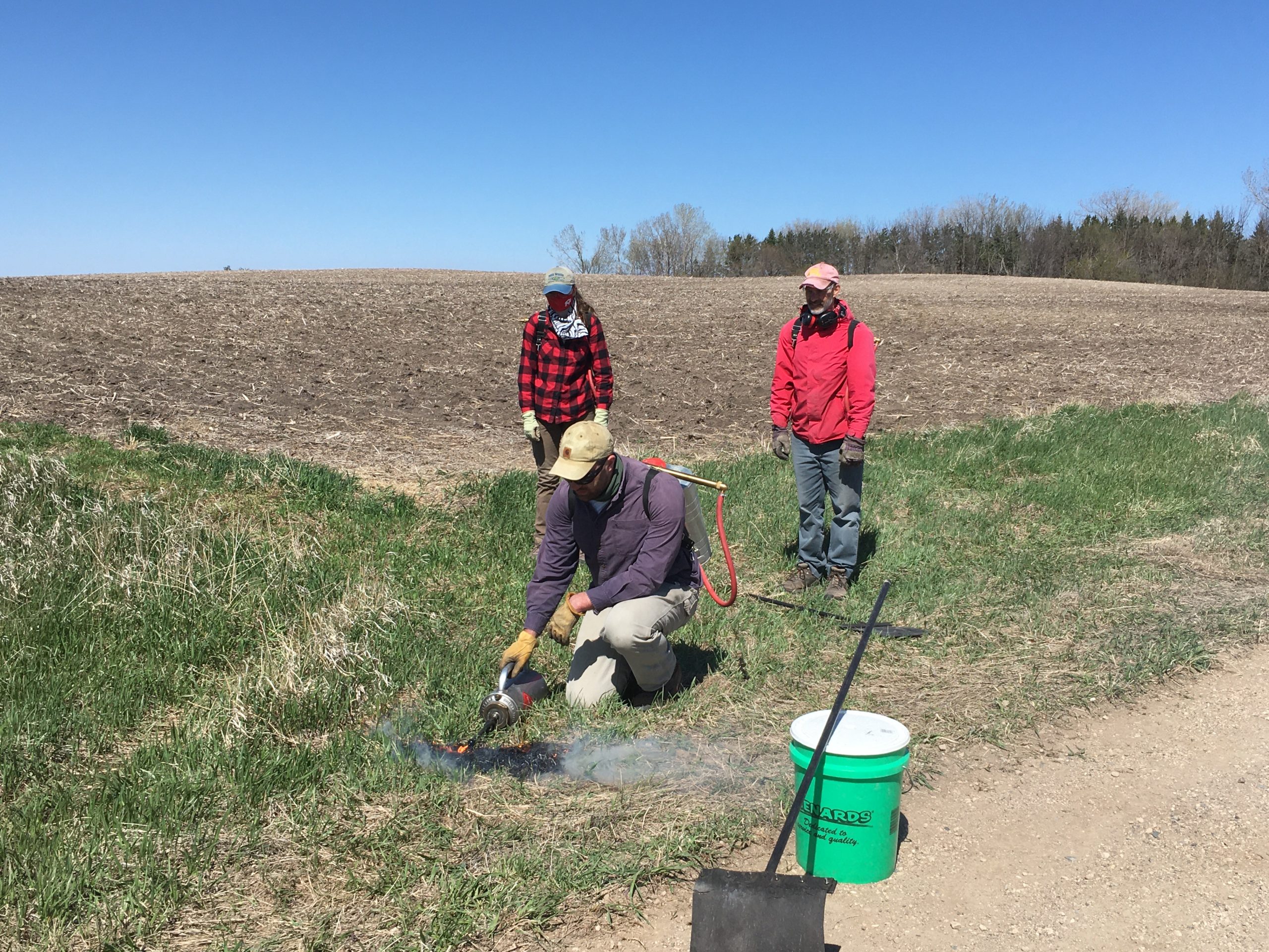
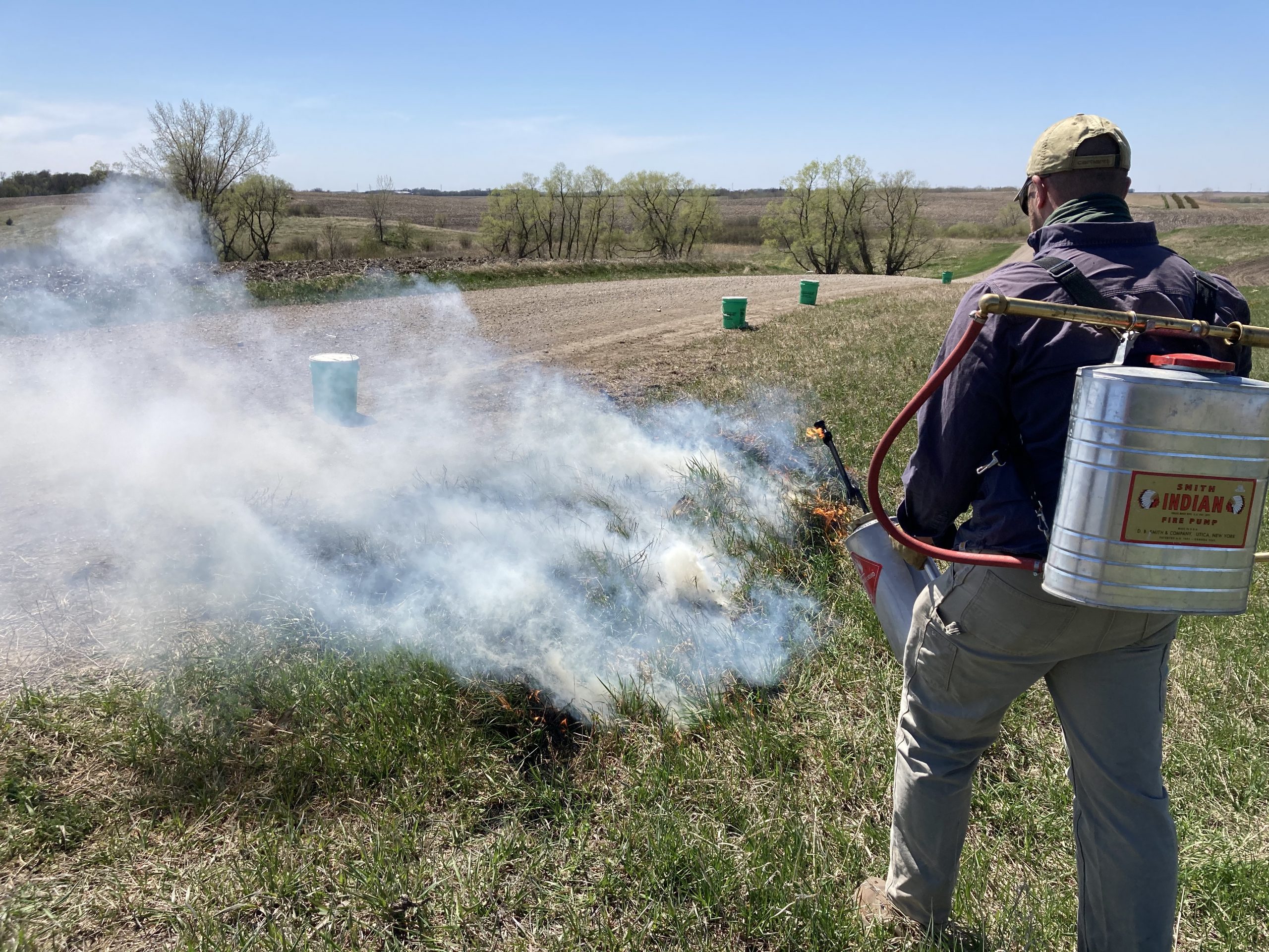
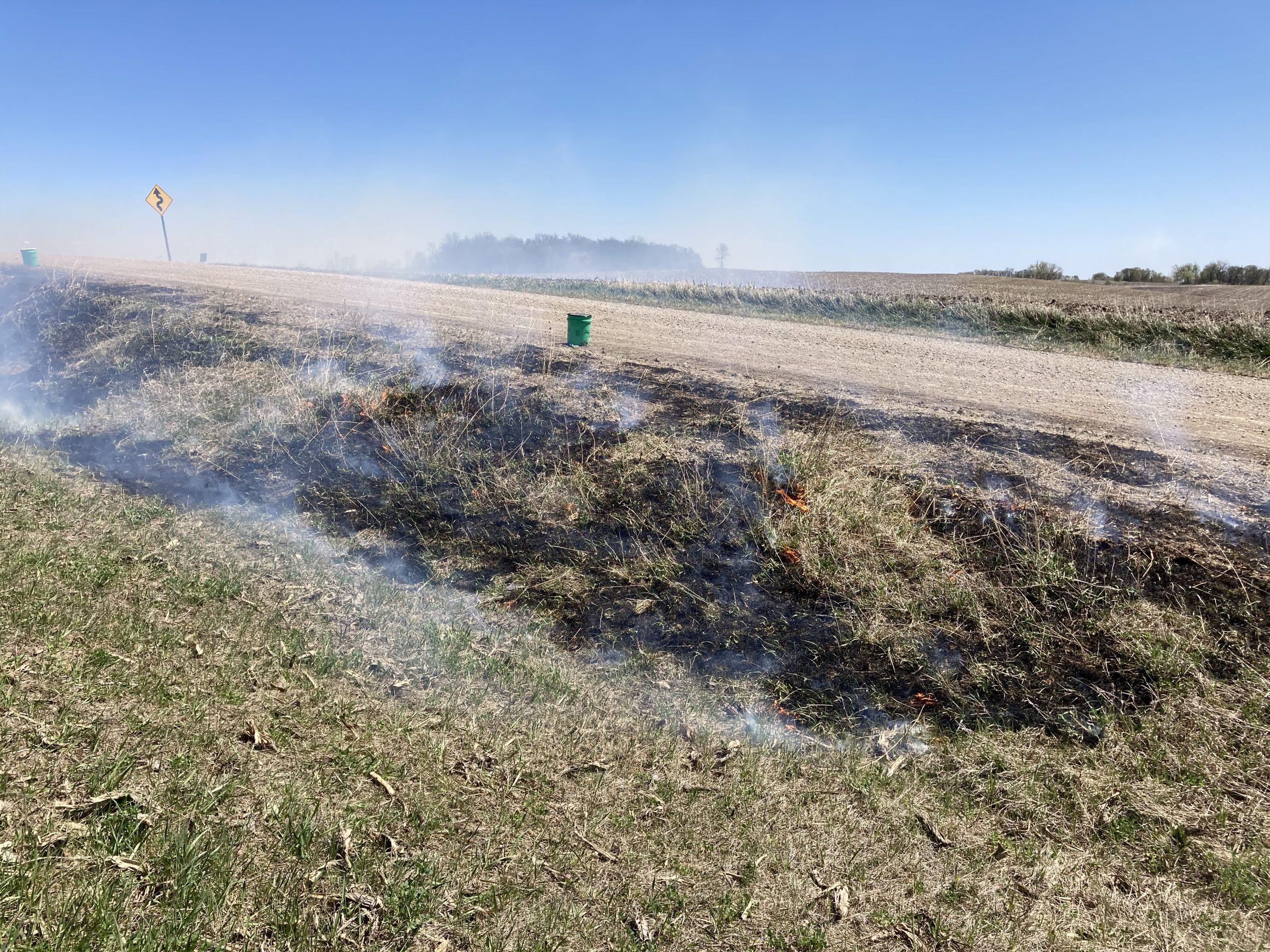
Weather conditions Tuesday afternoon were favorable for burning but wind forecasts were at the upper end of our burn prescription. Given our success burning p8 in similar conditions just a week earlier, we decided to proceed cautiously by starting with a prescribed burn on the north side of east riley. Here light and discontinuous fuel (mostly brome), a gravel road for a firebreak on the south side, and agricultural fields downwind mitigated our concerns about gusty winds. Earlier in the day, Mia mowed fire breaks along the east and west end of the burn unit. We ate lunch, loaded up our equipment, and drove down to east riley. Along the way, the crew got a great look at a western kingbird perched along Sandy Hill Road.
Once at the site, we reviewed the burn plan and staged equipment. We ignited a test fire in the southeast corner of the burn unit. Despite a slow start to the test fire and stiff NW winds that kept extinguishing the drip torch, the backing fire burned well through brome and scattered warm season grasses. With scattered poison ivy in the eastern third of east riley, we were cautious to stay upwind of smoke by lighting small strips perpendicular to the wind. Once sufficient black (burned area downwind) had been established, we proceeded to ignite the southern edge of the unit along Mellow Ln and wrap around the western end of the unit to ignite a head fire along the northern edge of the burn unit.
While somewhat patchy, we considered the burn a success. The fire behaved predictably and we felt comfortable that we could continue burning other units with more fuel. After the burn, Stuart shared the observation that the fire did not carry well in areas where fuel was covered by a film of silt/gravel. We packed up and drove a short distance into Grant County for our next set of burn units…
Temperature – 52 F Relative humidity – 34% Wind speed (max gusts) – 13 (22) mph wind direction – NNW Ignition time – 2:22 PM End time – 2:58 PM Burn crew: Jared, Stuart, Gretel, Mia
Before and after comparison looking west along Mellow Ln.
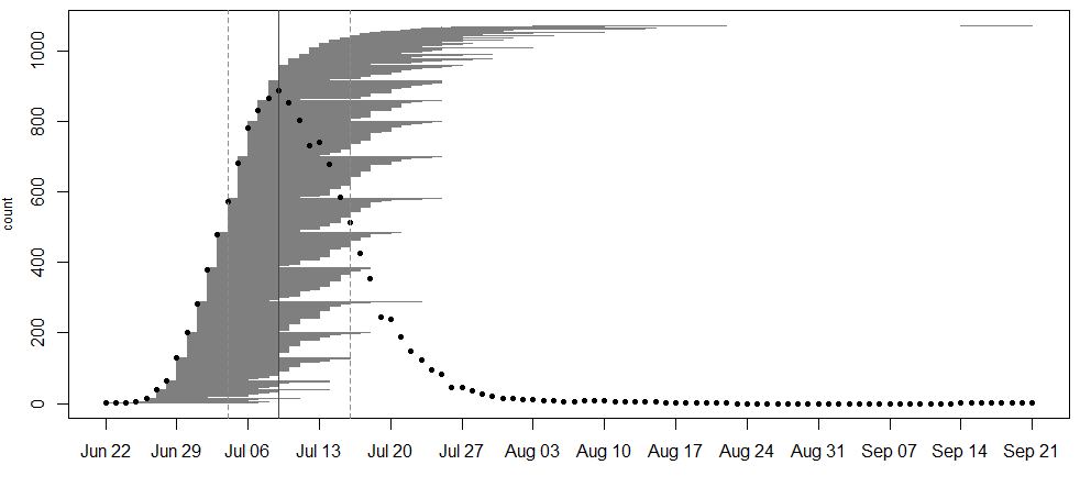
In 2020, we collected data on the timing of flowering for 855 flowering plants (1071 flowering heads) in 31 remnant populations. The plants ranged from having 1 to 8 flowering heads. The earliest bloomers initiated flowering on June 22nd . Plant 22195 at NWLF was the latest bloomer, only beginning to shed pollen on September 14th, nearly a month after the second-latest flowering plant had ceased producing pollen (August 18th). As is typical for the latest bloomer of a season, township mowers had mowed over this plant earlier in the season, which is perhaps why it took longer for it to sprout a new flowering stem. Peak flowering was on July 9th, when 886 heads were flowering.
A major part of the motivation behind this year’s effort in monitoring phenology was to collect baseline data on flowering rates and timing. Team Echinacea recently received funding to perform prescribed burns in these populations. Next summer, we will compare flowering patterns in populations before and after fires to understand how burns drive the effects of timing of flowering on mating patterns and fitness of individuals in natural populations.
Start year: 1996
Location: Roadsides, railroad rights of way, and nature preserves in and around Solem Township, MN
Overlaps with: phenology in experimental plots, demography in the remnants, gene flow in remnants, reproductive fitness in remnants
Data/materials collected: We identify each plant with a numbered tag affixed to the base and give each head a colored twist tie, so that each head has a unique tag/twist-tie combination, or “head ID”, under which we store all phenology data.We monitor the flowering status of all flowering plants in the remnants, visiting at least once every three days (usually every two days) until all heads were done flowering to obtain start and end dates of flowering. We managed the data in the R project ‘aiisummer2020′ and will add the records to the database of previous years’ remnant phenology records, which is located here: https://echinaceaproject.org/datasets/remnant-phen/. The dataset is ready to be updated, but I don’t believe it has been at the time of writing.
A flowering schedule for individuals from all remnants. Notice the gap between when second-to-last flower ceased pollen production and when the latest bloomer began on September 14th!
A flowering curve (created here using the R package mateable) summarizes the flowering phenology data that we collected in 2020, indicating the number of individuals flowering on a given day and the flowering period for all individuals over the course of the season.
We shot GPS points at all of the plants we monitored. Soon, we will align the locations of plants this year with previously recorded locations and given a unique identifier (‘AKA’). We will link this year’s phenology and survey records via the headID to AKA table.
You can find more information about phenology in the remnants and links to previous flog posts regarding this experiment at the background page for the experiment.
Products: A dataset of flowering phenology is ready to be posted on the website. It is currently located in Dropbox\remData\105_assessPhenology\phenology2020\phen2020_out and is available upon request. The headIds in this dataset have not yet been merged with the akas (long-term identifiers) in the demography dataset.
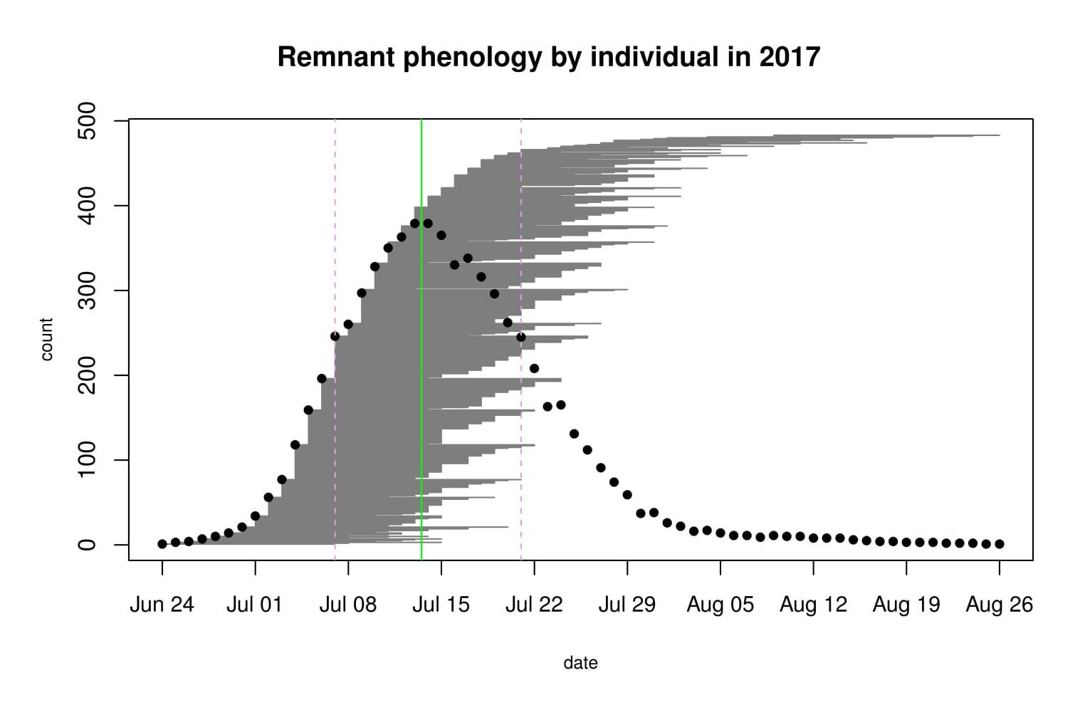
In 2019,
we collected data on the timing of flowering for 95 flowering plants (127
flowering heads) in 8 remnant populations, which ranged from 1 to 29 flowering heads.
The earliest bloomers (four plants at four different remnants) initiated
flowering on July 4. Plant 24050 in the aptly named remnant population North of
Northwest of Landfill was the latest bloomer, shedding its last anthers of
pollen on August 16. Township mowers had mowed over this plant earlier in the
season, which is perhaps why it took longer for it to sprout a new flowering
stem. Altogether, the flowering season was 43 days long. Peak flowering was on
July 19, when 105 heads were flowering.
This season
marked the 19th season of collecting phenology records in remnant populations! Though
we do not have data for all populations every year, Stuart monitored phenology
in all of our remnant populations in 1996 and in following years (2007, 2009,
2011-2019) students and interns studied phenology in particular populations. From
2014-2016, determining flowering phenology was a major focus of the summer
fieldwork, with Team Echinacea tracking phenology in all plants in all of our
remnant populations. The motivation behind this study is to understand how
timing of flowering affects the mating patterns and fitness of individuals in
natural populations.
Flowering
occurred much later this season than previous years, with peak flowering
falling a full 14 days later in the year than 2018, when flowering started on
June 20, and 10 days later than 2017. Of all the years that we data for flowering
phenology in the remnant populations in and around Solem Township, this season was
the second-latest, with only the 2013 season beginning later, on July 6.
However, this observation comes with the caveat that sampling effort varied
between years and some years focused on particular contexts, such as population
where a portion had experienced a spring burn (see Fire and Flowering at SPP). Many other plants and animals in
Minnesota seemed to have delayed phenology this spring and summer, perhaps a
result of an unusually wet and snowy spring.
Start
year: 1996
Location: Roadsides,
railroad rights of way, and nature preserves in and around Solem Township, MN
Overlaps
with: phenology in experimental plots, demography in the
remnants, gene flow in remnants, reproductive fitness in remnants
Data/materials
collected:We identify each plant with a numbered tag affixed to
the base and give each head a colored twist tie, so that each head has a unique
tag/twist-tie combination, or “head ID”, under which we store all phenology
data.We monitor the flowering status of all flowering plants in
the remnants, visiting at least once every three days (usually every two days)
until all heads were done flowering to obtain start and end dates of flowering.
We managed the data in the R project ‘aiisummer2019′ and added the records to
the database of previous years’ remnant phenology records, which is located
here: https://echinaceaproject.org/datasets/remnant-phen/.
A flowering curve (created here using the R package mateable) summarizes the flowering phenology data that we collected in 2019, indicating the number of individuals flowering on a given day and the flowering period for all individuals over the course of the season.
We shot
GPS points at all of the plants we monitored. Soon, we will align the locations
of plants this year with previously recorded locations and given a unique
identifier (‘AKA’). We will link this year’s phenology and survey records via
the headID to AKA table.
We
harvested a random sample of 1/3 of the flowering heads from each remnants in
August and September, plus an X additional heads from populations that were highly
isolated, for a total of X harvested seedheads. These are currently stored at
the University of Minnesota. This winter, I will assess the relationship
between phenology and reproductive fitness by x-raying all of the seeds we collected.
In addition, I will determine the paternity (i.e., pollen source) for a sample
of seeds by matching the seed genotype to the potential pollen donors. Doing so
will shed light on how phenology influences pollen movement and gene flow
patterns.
You can
find more information about phenology in the remnants and links to previous
flog posts regarding this experiment at the background
page for the experiment.
Products: I presented a poster based on the
locations and flowering phenology of individuals from summer 2018 at the
International Pollinator Conference in Davis, CA this summer. The poster is
linked here: https://echinaceaproject.org/international-pollinator-conference/.
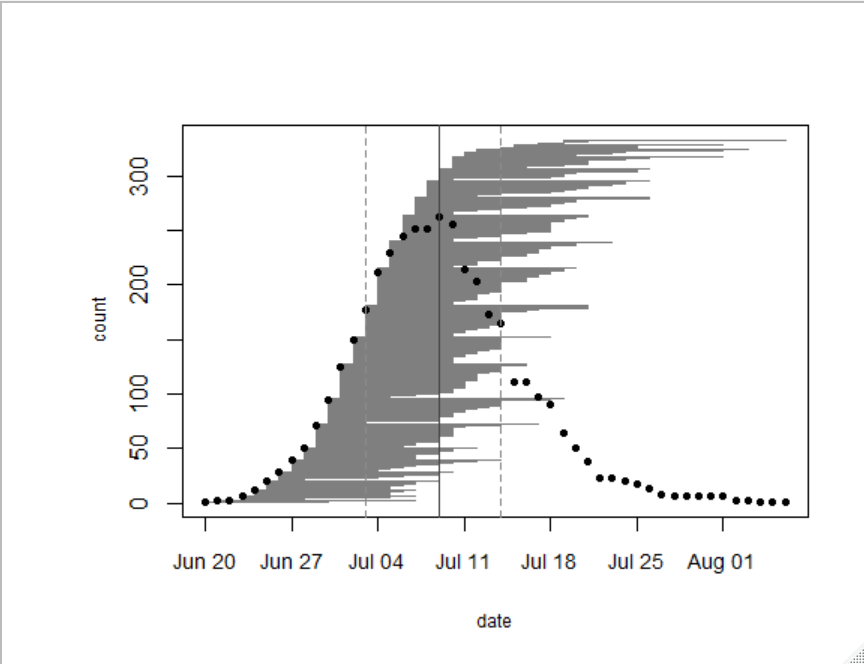
In 2018, we collected data on the timing of flowering in 333 individual plants growing in our naturally occurring prairie remnants: 119 plants at Staffanson Preserve and 214 at others remnants. Flowering began on June 20th – four days earlier than last year. The last date of flowering was on August 9th – the latest bloomer was a roadside plant that had been mowed early in the season but put up another stem later in the season. Peak flowering for the remnants we observed in 2018 was on July 9th, which again was 4 days earlier than 2017. That day there were 257 individuals flowering. The figure below was generated with R package mateable, which was was developed by Team Echinacea to visualize and analyze phenology data.
From 2014-2016, determining flowering phenology was a major focus of the summer fieldwork, with Team Echinacea tracking phenology in all plants in all of our remnant populations. Stuart began studying phenology in remnant populations in 1996, but he didn’t know that keeping track of the dates was called “phenology.” In following years, several students & interns also studied phenology in certain populations. The motivation behind this study is to understand how timing of flowering affects the reproductive opportunities and fitness of individuals in natural populations.
Start year: 1996
Location: roadsides, railroad rights of way, and nature preserves in and near Solem Township, MN
Amy Waananen harvested some heads in fall 2018 and is germinating seeds right now at the U of MN. She is keeping track of which plant (mom) each seedling came from. She aims to use DNA fingerprinting techniques to identify the pollen donor (dad) of each seedling to get a sense of how far pollen moves in fragmented prairie habitat.
Data collected: We identify each plant with a numbered tag affixed to the base and give each head a colored twist tie, so that each head has a unique tag/twist-tie combination, or “head ID”, under which we store all phenology data.We monitor the flowering status of all flowering plants in the remnants, visiting at least once every three days (usually every two days) until all heads were done flowering to obtain start and end dates of flowering. We managed the data in the R project ‘aiisummer2018′ and will add it to the database of previous years’ remnant phenology records. Ask Amy Waananen for more specific data regarding phenology in the 2017 and 2018 seasons.
GPS points shot: We shot GPS points at all of the plants we monitored. The locations of plants this year will be aligned with previously recorded locations, and each will be given a unique identifier (‘AKA’). We will link this year’s phenology and survey records via the headID to AKA table. Ask Amy Waananen for more specific data regarding phenology in the 2017 and 2018 seasons.
You can find more information about phenology in the remnants and links to previous flog posts regarding this experiment at the background page for the experiment.
For her REU project, Brigid gathered data to study the relationship between flowering density and seed set. She worked at Staffanson Prairie Preserve, which appears to have higher flowering density in burn years than non-burn years. This year, 2018, was a burn year on the east side of the preserve. Brigid and Team Echinacea kept track of the style persistence of about ~150 individuals many of which we have phenology and style persistence information from prior years. These individuals were harvested and their achene count and seed set will be assessed by volunteers and interns at the CBG.
Brigid also observed nearest neighbors for many of the plants that she tracked. It might be the cases that echinacea flowers are more successful if they have other flowering plants nearby. Synchrony is a large part of why fire is so important, and, since SPP is our largest remnant prairie, it’s the best place to test the relationship between fire and synchrony. Number of heads, phenology, and head size may also \ interact with fire — we’ll know once we look at the data!
Data and Samples: We shot 90 GPS points for nearest neighbors, many of which were plants that flowered for the first time this year. We also harvested 22 heads that are awaiting cleaning at CBG
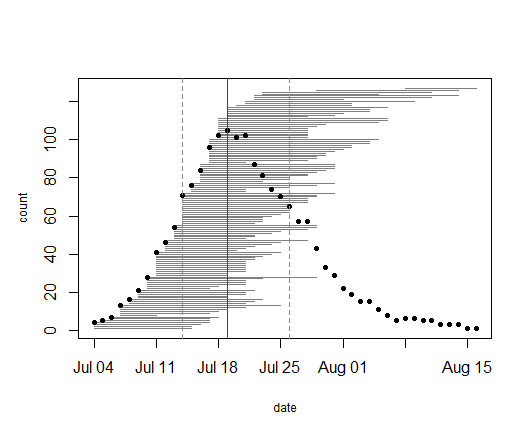
In 2017, according to our preliminary data, flowering began on June 24th with one head at the Aanenson remnant. The latest bloomer was a 5-headed plant at Steven’s Approach, and the last day its last head shed pollen was August 26th. Peak flowering for the 9 remnants we observed this year was July 13th. There was a total of 427 flowering plants producing 575 flowering heads. The figure below was generated with R package mateable, which was was developed by Team Echinacea to visualize and analyze phenology data.
The gray shaded area is made up of horizontal gray lines, each representing the duration of one flowering head. The vertical green line represents the peak flowering date, July 13th. On average, heads flowered for approximately 2 weeks.
From 2014-2016, determining flowering phenology was a major focus of the summer fieldwork, with Team Echinacea tracking phenology in all plant in all of our remnant populations. Stuart began studying phenology in remnant populations between 1996 and 1999 and several students also studied certain populations in following years. The motivation behind this study is to understand how timing of flowering affects the reproductive opportunities and fitness of individuals in natural populations.
Start year: 1996
Location: roadsides, railroad rights of way, and nature preserves in and near Solem Township, MN (2017: Aanenson, Around Landfill, East Elk Lake Road, Nessman, Northwest Landfill, Steven’s Approach, Staffanson Prairie Preserve, Town Hall)
Overlaps with: Phenology in experimental plots, demography in the remnants, reproductive fitness in remnants
Physical specimens:
We harvested 121 Echinacea heads at 8 of the 28 remnants. These were harvested from Lea and Tracie’s “rich hood” (richness of neighborhood) plots. Not all harvested heads were monitored for the phenology dataset.
Data collected: We identify each plant with a numbered tag affixed to the base and give each head a colored twist tie, so that each head has a unique tag/twist-tie combination, or “head ID”, under which we store all phenology data.We monitor the flowering status of all flowering plants in the remnants, visiting at least once every three days (usually every two days) until all heads were done flowering to obtain start and end dates of flowering. We managed the data in the R project ‘aiisummer2017′ and will add it to the database of previous years’ remnant phenology records.
GPS points shot: We shot GPS points at all of the plants we monitored. The locations of plants this year will be aligned with previously recorded locations, and each will be given a unique identifier (‘AKA’). We will link this year’s phenology and survey records via the headID to AKA table.
You can find more information about phenology in the remnants and links to previous flog posts regarding this experiment at the background page for the experiment.
For the past three years, studying phenology in the remnants has been a major focus of our summer field work. The motivation behind this study is to understand how timing of flowering affects the reproductive opportunity and fitness of individuals in natural populations. Stuart began studying phenology in remnant populations between 1996 and 1999 and several students also studied certain populations in following years. From 2014-2016, we tracked phenology in all of our remnant populations. This year there were 1040 flowering plants (1500 flowering heads).
Flowering began on June 18th with one plant at the East Riley roadside remnant. Sadly, this early bloomer was mowed just 6 days after it started flowering. The latest flowering plant shed pollen in the West Unit of Staffanson Prairie Preserve on August 17th. When we consider all populations together, peak flowering was on July 10th. Peak flowering at Staffanson Prairie Preserve was later, on July 18th, likely due to the prescribed burn in the West Unit setting flowering back.
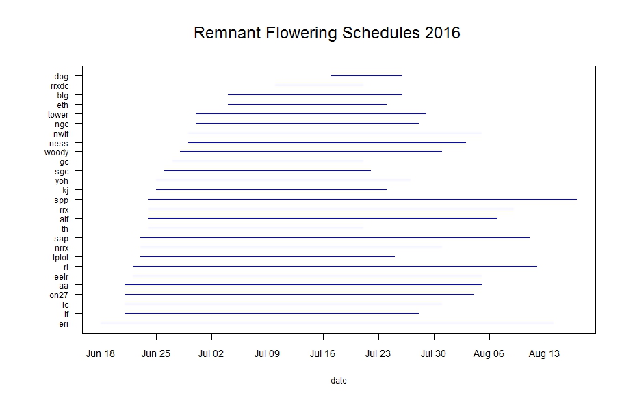
Line segments represent the duration of flowering for each remnant population. Click to enlarge!
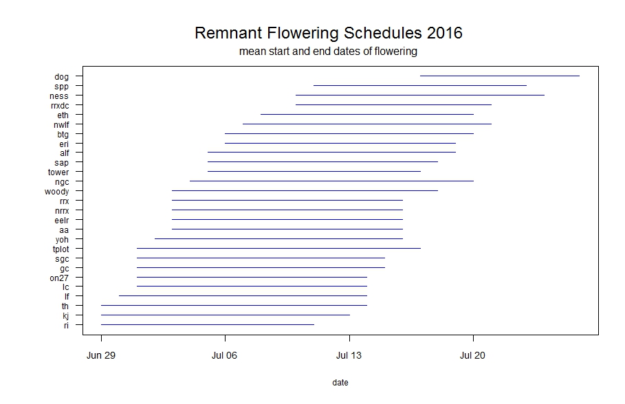
As you can see in the figure above, some populations had much longer duration of flowering than others. Flowering duration at Staffanson Prairie Preserve (‘spp’ in the figure) was longer because the west unit was delayed in flowering. East Riley (‘eri’) has a long duration of flowering, likely due to individuals being mowed early in the season, then resprouting and flowering later. This figure shows the very first and last dates of flowering, but population mean start and end dates of flowering is also informative (see what that flowering schedule looks like here). These figure with generated with R package mateable, which was was developed by Team Echinacea to visualize and analyze phenology data.
Start year: 1996
Location: roadsides, railroad rights of way, and nature preserves in and near Solem Township, MN
Overlaps with: Phenology in experimental plots, demography in the remnants
Physical specimens:
We harvested a random sample of 5 heads from most remnant populations (we excluded very small populations) and brought them back to the lab, where student interns will process and assess their seed set (‘regRem’ or ‘regular remnant harvest’).
We also harvested the most isolated, least isolated, earliest flowering, and latest flowering individuals from large populations (‘remnant extremes’). Student interns will also process and assess seed set of these heads.
Data collected: We identify each plant with a numbered tag affixed to the stem and give each head a differently colored twist tie, so that each head has a unique tag/twist-tie combination, or “head ID”, under which we store all phenology data.We monitor the flowering status of all flowering plants in the remnants, visiting at least once every three days until all heads were done flowering to obtain start and end dates of flowering. We managed the data in the R project ‘aiisummer2016′ and will add it to the database of previous years’ remnant phenology records.
GPS points shot: We shot GPS points at all of the plants we monitored except for four, two at SGC and two at ERI, which were mowed (ERI) or dug up (SGC) early in the season. These points were shot under job names following the convention “SURV_2016MMDD_SULU” or “SURV_2016MMDD_CHEK”. The locations of plants this year will be aligned with previously recorded locations, and each will be given an identifier (‘AKA’). We will link this year’s phenology and survey records via the headID to AKA table.
You can find more information about phenology in the remnants and links to previous flog posts regarding this experiment at the background page for the experiment.
So it begins! Two new externs have joined Team Echinacea from Carleton College. We (Mikaela and Emma) will be here every day for the next three weeks, and are excited to discover new revelations for the Asynchrony, Isolation and Incompatibility experiment.
So far, most of what we’ve discovered is that cleaning Echinacea seed heads is tedious. Two days in, we have cleaned 36 seed heads; scanning them was a nice relief from the monotony. We think we could get through all 110 by the end of this week.
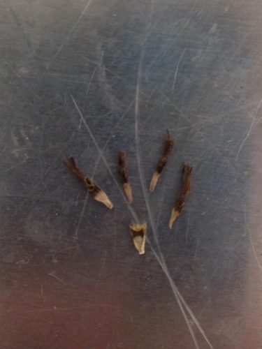
Although yesterday was quiet, there was a little bit of commotion: Mikaela’s second seed head had a rare deformity. Many of the achenes were uninformative. This means they were aborted part of the way through formation, so it cannot be determined whether they were fertilized. After minutes of puzzled deliberation, Stuart, Amy and Scott decided to keep them in the sample.
Four uninformative achenes compared to one normal, small-to-mid-size achene. Because of their immaturity, the florets are still firmly attached.
In contrast to yesterday, today there were quite a few volunteers and a couple of students who we got to meet. It was nice to talk to other people who were involved in and excited about this project. We also got to hear about other experiments going on in the lab besides our own.
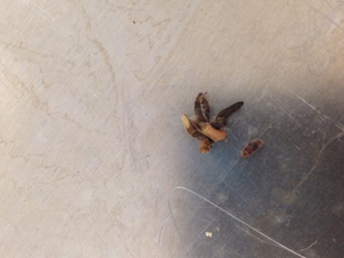
Today’s seed cleaning also presented an exciting moment: just moments after Amy told us about last year’s larval discoveries, we each found a live larva residing in the heads we were cleaning. We’re thinking about raising these mystery larva so we can finally learn just what they are. Hopefully we’ll have more success than last year’s effort!
Our two larva. Emma’s is the tiny brown one on the right, and Mikaela’s is the pink one hanging out on a makeshift habitat of chaff.
We are grateful for this opportunity to contribute to and learn from the project, and are looking forward to the next three weeks!
Last time I mentioned in passing that Stuart, Amy, Scott, and I had been discussing papers about fire and its potential impact on the reproductive fitness on Echinacea plants. This week I will go into greater detail about what I’ve learned about fire and what our data can teach us about how it impacts prairie health.
Some of our studies taken from previous years have shown us that, even when there are enough bees to carry pollen from plant to plant, Echinacea plants can have difficulties receiving pollen from potential mates. There are a few reasons for this. In our fragmented prairie remnants, Echinacea plants are often far enough apart that pollen collected by a bee will often fall off before it can reach another Echinacea flower. Echinacea plants may also flower in different years, or at different times in the season. This can prevent mating even between close flowers. This mate availability problem is compounded by the fact that Echinacea is self-incompatible, meaning a plant cannot pollinate itself or its close relatives. This means that if a plant flowers and fails to find mates, all the energy it expends to flower and fruit results in no offspring. This is an extraordinary energy cost for no payoff.
Data we have collected seems to suggest that fires may help perennial prairie plants like Echinacea find other mates. Explosive flowering after a large burn is typical for prairie plants. There is some evidence that increased availability of nutrients from burned organic matter and the increased availability of sunlight provide resources for a plant to invest in a costly reproductive structure like a flower. This is probably no different for Echinacea. However, as an added bonus, some of our data seems to show that this explosive flowering may reduce the reproductive isolation of Echinacea plants by increasing the number of synchronous flowering plants. Thus, fire helps Echinacea successfully seed by increasing the number of available mates. Really cool!
The tendency of Echinacea to flower synchronously after a fire could be the result of natural selection, or simply a byproduct of the excellent growing conditions created by fire. In either case, this knowledge affirms how important fires are to prairie ecosystems. The Echinacea Project, through projects like SppBonus, hopes to further elucidate these mechanisms through which fire improves prairie health.
Until next time!
Sam
Citations:
Wagenius, S. and Lyon, S. P. (2010), Reproduction of Echinacea angustifolia in fragmented prairie is pollen-limited but not pollinator-limited. Ecology, 91: 733–742. doi:10.1890/08-1375.1
Ison, J.L., S. Wagenius, D. Reitz., M.V. Ashley. 2014. Mating between Echinacea angustifolia (Asteraceae) individuals increases with their flowering synchrony and spatial proximity. American Journal of Botany 101: 180-189.


