|
|
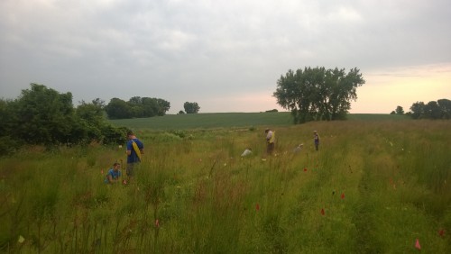
 Team Echinacea measuring plants in big batch The qGen1 (quantitative genetics) experiment is designed to quantify the heritability of traits in Echinacea angustifolia. We are especially interested in Darwinian fitness. Could fitness be heritable? During the summer of 2002 we crossed plants from the 1996 & 1997 cohorts of exPt1. We harvested heads, dissected achenes, and germinated seeds over the winter. In the Spring of 2003 we planted the resulting 4468 seedlings (this great number gave rise to this experiment’s nickname “big batch”). In 2016 we assessed survival and fitness measures of the qGen1 plants. 2,187 plants in qGen1 were alive in 2016. Of those, 5% flowered in 2016 and 49% have yet to flower.
Start year: 2003
Location: Experimental plot 1
Overlaps with: qGen2 & qGen3
Physical specimens: We harvested 116 heads from qGen1 in 2016. These heads will be processed in the lab to determine achene count and seed set.
Data collected: We collected fitness measures using handheld computers.
Products: We have an awesome dataset that we will share once the paper is published. Ruth Shaw is working on an analysis of the qGen1 dataset.
You can find more information about Heritability of fitness–qGen1 and links to previous flog posts regarding this experiment at the background page for the experiment.
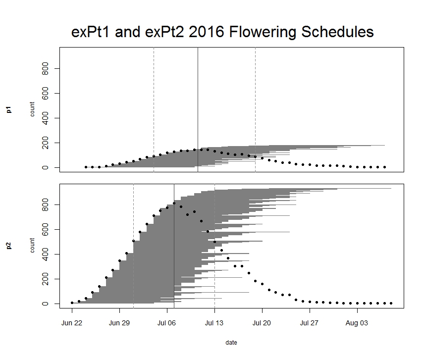
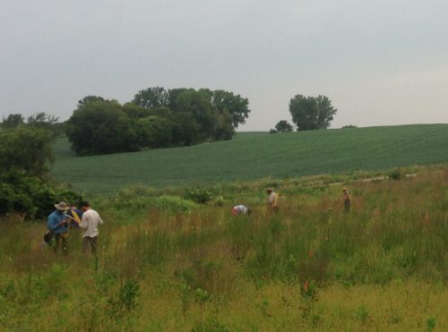
Every year we keep track of flowering phenology in our main experimental plots, exPt1 and exPt2. Fewer plants than usual flowered in exPt1 in 2016: 149 plants (179 heads) flowered between June 24th and August 7th. The population’s mean start date of flowering was July 5th and the mean end date was July 18th. Peak flowering in 2016 was on July 10th, when 143 heads were in flower. For comparison, peak flowering in 2015 was on July 27th, when there were nearly 10x as many heads flowering as on this year’s peak. The earlier phenology and low numbers of flowering we observed this year relative to 2015 is likely due at least in part to the plot burn schedule (2015 was a burn year and 2016 was a non-burn year), but there were still many fewer flowering plants than any season, burn or non-burn, in the past 10 years.
We kept track of 934 flowering heads in ExPt2, where the first head started shedding pollen on June 22 and the latest bloomer ended flowering on August 8th. Peak flowering was on July 7th, when 810 heads were flowering. ExPt2 was designed to study the heritability of phenology—you can read more about progress of that experiment in the upcoming 2016 heritability of phenology project status update.
At the end of the season we harvested the heads and brought them back to the lab, where we will count fruits (achenes) and assess seed set.
 ExPt1 and Expt2 flowering schedules from 2016. Dots represent the number of flowering heads on each date. Horizontal line segments represent the duration of each heads flowering and are ordered by start date. The solid vertical line indicates peak flowering, while the dashed lines indicate the dates when 25% and 75% of heads had begun flowering, respectively. Click to enlarge! Start year: 2005
Location: Experimental Plots 1 and 2
Overlaps with: Heritability of flowering time, common garden experiment, phenology in the remnants
Physical specimens: We harvested 177 heads from exPt1 and 870 from exPt2. Attentive readers may note that we harvested about 64 fewer heads than we tracked for phenology. That’s because before we could harvest many seedheads at exPt2, rodents chewed through their stems and ate some fruits (achenes). We recovered most of the heads that were grazed from the ground and made estimates of number of fruits lost due to herbivory, but we couldn’t find some heads. Arg. We brought the harvest back to the lab, where we will count fruits and assess seed set.
Data collected: We visit all plants with flowering heads every three days until they are done flowering to record start and end dates of flowering for all heads. We managed phenology data in R and added it to the full dataset. The figure above was generated using package mateable in R. If you want to make figures like this one, download package mateable from CRAN!
You can find more information about phenology in experimental plots and links to previous flog posts regarding this experiment at the background page for the experiment.
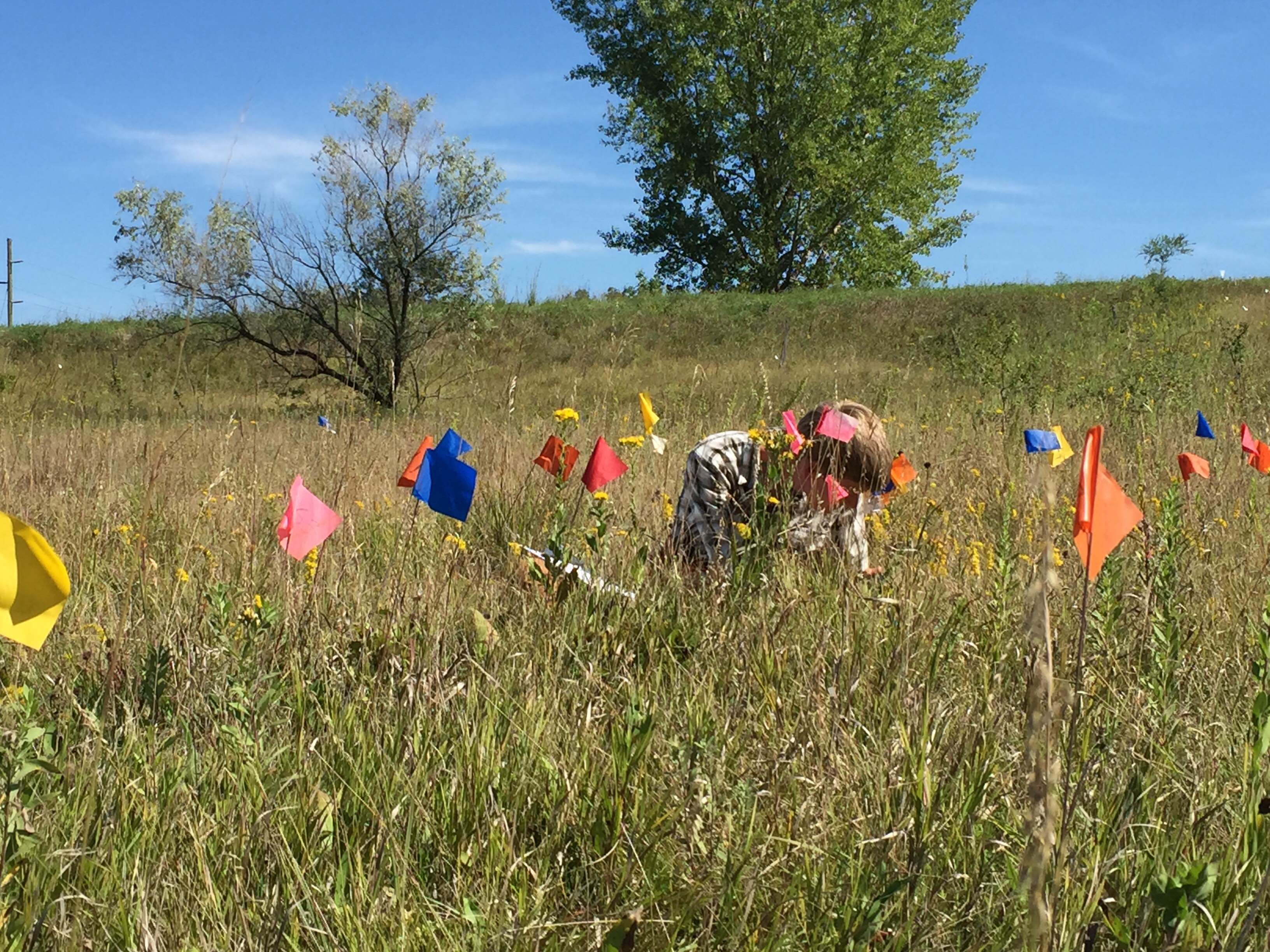
 We revisited locations in remnants where flowering plants were observed in previous years. We tag each Echinacea plant we see flowering in our prairie remnants, and record its location using the GPS. This is useful because it allows us to revisit the same plant in future years, checking to see if it is still alive, and if so how large it is and whether or not it is flowering. This has provided us with a very rich longitudinal dataset of life histories, dating back two decades and including thousands of plants. This year, we did total demo, visiting each plant in our database, at several sites including Staffanson, Loeffler’s Corner East, Northwest of Landfill, and East Elk Lake Road. In the interest of time, we only did flowering demo (only visiting plants that flowered this year) at several sites, including Landfill, Around Landfill, and Railroad Crossing. For each plant visited, we recorded its status (e.g., basal, flowering), its number of rosettes, and any neighboring Echinacea within a 12 cm radius. This data can be used to study inter-annual variation in flowering, population dynamics, and response to fire.
Year: 1996
Location: Roadsides, railroad rights of way, and nature preserves in and near Solem Township, Minnesota.
Overlaps with: Flowering phenology in remnants, fire and flowering at SPP
Data collected: Flowering status, number of rosettes, number of heads, neighbors within a 12 cm radius of plants found, stored in demo2016
GPS points shot: Points for each flowering plant this year shot mostly in PHEN records, stored in surv.csv. Some points of flowering plants stored in SURV records, also in surv.csv. Each location should be either associated with a loc from prior years or a point shot this year.
Products:
- Amy Dykstra’s dissertation included matrix projection modeling using demographic data
- Project “demap” merges phenological, spatial and demographic data for remnant plants
You can find out more about the demographic census in the remnants and links to previous posts regarding it on the background page for this experiment.
Hey Flog readers, Sam here.
After a quarter of hard work, all of the achenes from my thirty-two flowerheads have been counted, x-rayed, and classified! I am looking forward to analyzing the data next quarter in R through a class Stuart teaches at Northwestern. It’s been quite a journey learning about both the nitty-gritty of going from flower head to data sheet and the conservation biology through which we contextualize our data. Special thanks to Stuart for giving me the opportunity to intern for the Echinacea project, to Amy and Scott for being wonderful, helpful mentors, and to everyone else in the lab for your amazing company and support. If anyone reading this would like to know more about what it is like to intern for the Echinacea Project, feel free to e-mail me at Samuelhamilton2017@u.northwestern.edu.
Best,
Sam
Hey again Flog,
My name is Sam Hamilton and this is my second post on the Flog. In my first post, I focused on the experimental goals of the SppBonus project, the kind of data we are measuring, and the project’s relevance to understanding reproductive success in fragmented prairie remnants. Today, I will talk about the progress I’ve made, and the methods I’ve used to move this project from seed head to data set.
The first step of this project was to extract the achenes from the seed heads. Flowers of the Aster family, including Echinacea, are compound flowers, many flowers that grow together to look like one large flower. In Echinacea, each of these flowers, regardless of whether it is pollinated or not, produces a fruit called an achene. By measuring how many achenes contain seeds, we can estimate how well a flower was pollinated in a given year. Thus, in a project like SppBonus, the first step is to extract the seeds from the seed head. The SppBonus data set contained 32 different seed heads, which took me roughly a month to completely clean and organize into samples taken from the top, middle, and bottom of each flower.
The second step is to scan all the gathered achenes so that we can count the total number of achenes. This is an important metric to measure the reproductive fitness of each Echinacea plant. This was a fairly fast process and it only took me three days to scan the achenes from each seed head.
The third step is randomization. We ultimately determine whether or not an achene contains a seed by X-ray. However, there are simply too many seeds to X-ray them all efficiently. Thus, we take a sample from our seeds, X-ray those, and then use that data to make assumptions about the seed set as a whole. We randomize our samples, to ensure our samples are representative of their populations. Without this step, we risk choosing achenes that are the easiest to count, or best fit our expectations of what the data will look like. Our randomization procedure involves pouring the seeds onto a grid where each cell is assigned a letter and a number. A second sheet has these letter and number combinations in a random order and we go down the list selecting from each cell until we’ve collected thirty achenes total. This is the part of the project I’m working on now!
When not working on SppBonus, I am spending my time reading and discussing papers about fire and its effects on pollination and germination with Stuart, Amy, and Scott. I learn a lot from listening, and it’s always interesting to hear their insights into the merits and flaws of each paper, as well as to watch them design new experiments from the ground up.
Hopefully I didn’t bore you, until next time!
Sam
We were curious about the average sizes of our various remnant populations so I did some quick calculations and created this csv. As you can see, landfill is quite large with a median of 315 individuals found per year, whereas sites like dog and mapp are tiny, with only 3 plants found per year. At dog, to the best of our knowledge, there are only 3 Echinacea to be found, so we have regularly gathered demographic info on all of them. It’s important to note that these numbers are preliminary, rough estimates. Sometimes we have to redo a site during the summer so there will be twice as many records (hence the right skewed means), most of the time we focus on only finding flowering plants, but in some years at certain sites (e.g. landfill in 2005 and 2007) we’ve attempted to find every single individual whether or not it was flowering. All that said, here are some histograms showing numbers of demography records at each site per year:
demoSizeGraphs
The Stipa Project — studying the effects of habitat fragmentation on the ecology and evolution of Stipa, a cool-season grass. In 2009 & 2010 we planted over 4,000 Stipa seeds in exPt 1. We’ve been put to the test trying to find our Stipa plants in a matrix of other grasses, but once they flower they are easy to spot. While we collected seed from Stipa in our common garden in 2014, our 2015 search for flowering Stipa plants was fruitless!
Read more about the Stipa experiment.
Read more about the natural history of Stipa.
Start year: 2009
Location: exPt1
 2015 measuring qGen1: finding EA in a sea of flowering big bluestem! The qGen1 (quantitative genetics) experiment investigates the heritability of traits in Echinacea angustifolia. During the summer of 2002 we crossed plants from the 1996 & 1997 cohorts of exPt1. We harvested heads, dissected achenes, and germinated seeds over the winter. In the Spring of 2003 we planted the resulting 4468 seedlings (this great number gave rise to this experiment’s nickname “big batch”). In 2015 we assessed survival and fitness measures of the qGen1 plants. Here’s a summary of what we found:
| living |
flowering |
headCount |
| 2319 |
409 |
793 |
Read more about the qGen1 experiment.
Start year: 2003
Location: exPt1
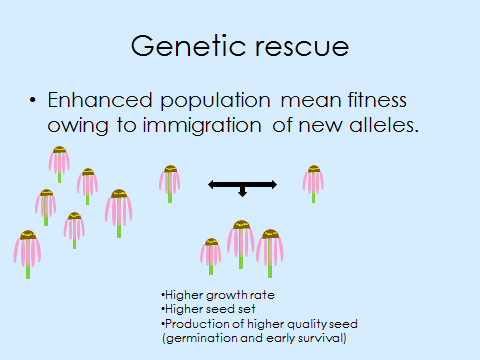
 Caroline Ridley established this experiment to compare fitness (recruitment and survival) of seeds originating from individuals with parents from three different backgrounds: 1. both from a large remnant population, 2. both from a small remnant population (not rescued), and 3. one from a large population and one from a small population (genetically rescued). Caroline sowed achenes in an experimental plot at Hegg Lake WMA and marked seedlings with colored toothpicks in May 2009. Caroline Ridley established this experiment to compare fitness (recruitment and survival) of seeds originating from individuals with parents from three different backgrounds: 1. both from a large remnant population, 2. both from a small remnant population (not rescued), and 3. one from a large population and one from a small population (genetically rescued). Caroline sowed achenes in an experimental plot at Hegg Lake WMA and marked seedlings with colored toothpicks in May 2009.
We annually assess survival and fitness of these plants. In 2015 we relocated and measured 42 individuals of the 381 seedlings originally found. These plants had 1-3 leaves; the longest leaf was 21 cm. The dense non-native brome grass dominating this plot may be shading out these small plants. It should be interesting to see which individuals are hanging on!
Read more about this experiment.
Start year: 2008
Site: exPt 4 at Hegg Lake WMA
Overlaps with: crossing experiments qGen1, qGen2, qGen3 & recruitment experiment; INB1
 Pollen vials from sire 403 used in qGen3 The goal of the qGen2 and qGen3 experiments is to compare the evolutionary potential of two remnant prairie populations of Echinacea angustifolia by estimating the additive genetic variance of fitness under two mating scenarios: crosses performed within the core sites (core x core) and crosses performed between the core site and nearby sites (core x periphery). Additionally, we will test for differentiation among families; do progeny from sires differ after accounting for maternal (dam) effects?
In June 2015 we assessed survival and measured 1-year-old plants from qGen2. During the summer and fall of 2015 we replicated the qGen2 experiment through a second crossing experiment. We sowed the resulting achenes in exPt 8 as our qGen3 cohort.
Read more about the qgen2 and qgen3 experiments.
Dam to be crossed with pollen from 2 sires Start year qGen2: 2013
Start year qGen3: 2015
Location: exPt 1 (dams), remnants Landfill and Staffanson (sires), remnants Landfill (core) & around Landfill (peripheral) and remnants Staffanson (core) & railroad crossing sites (peripheral) (grand-dams), exPt 8 (progeny)
Overlaps with: Heritability of fitness–qGen1
|
|


 Caroline Ridley established this experiment to compare fitness (recruitment and survival) of seeds originating from individuals with parents from three different backgrounds: 1. both from a large remnant population, 2. both from a small remnant population (not rescued), and 3. one from a large population and one from a small population (genetically rescued). Caroline sowed achenes in an experimental plot at Hegg Lake WMA and marked seedlings with colored toothpicks in May 2009.
