|
|
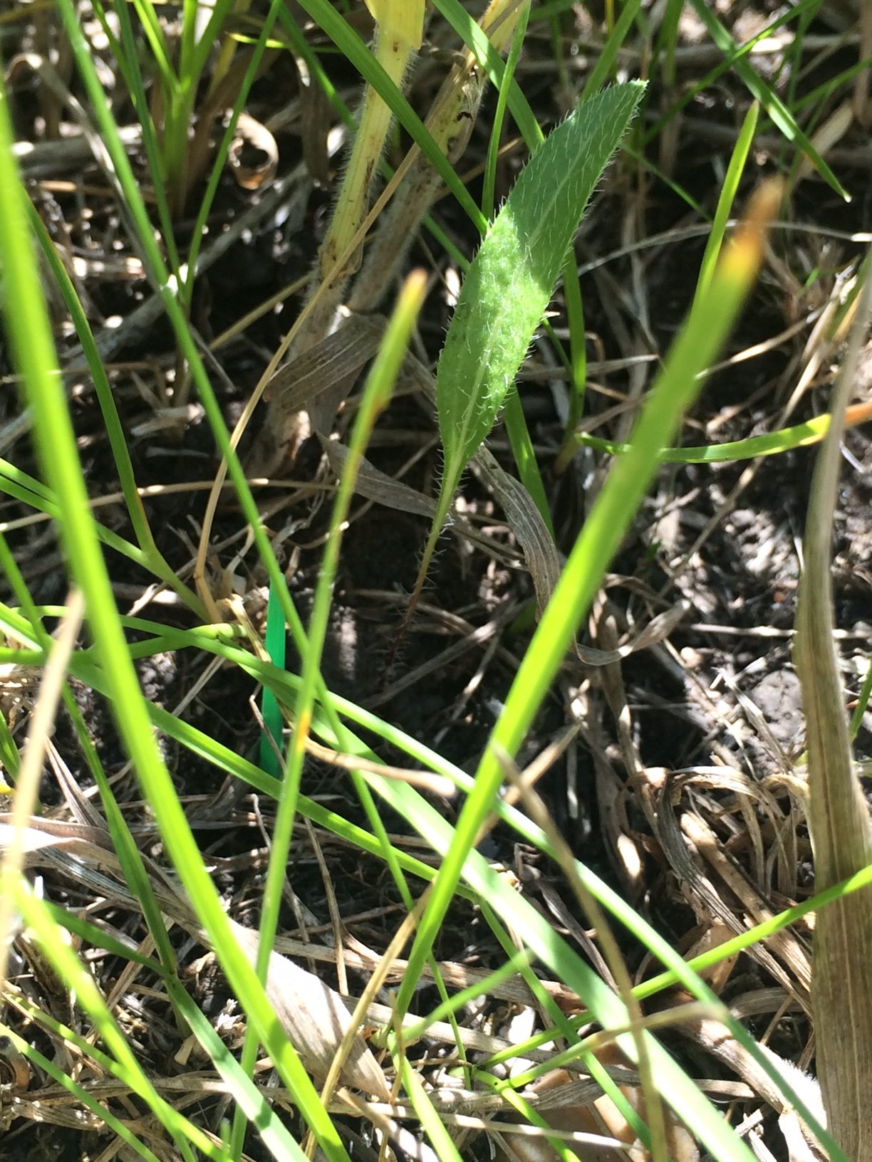
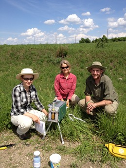
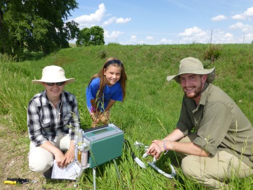
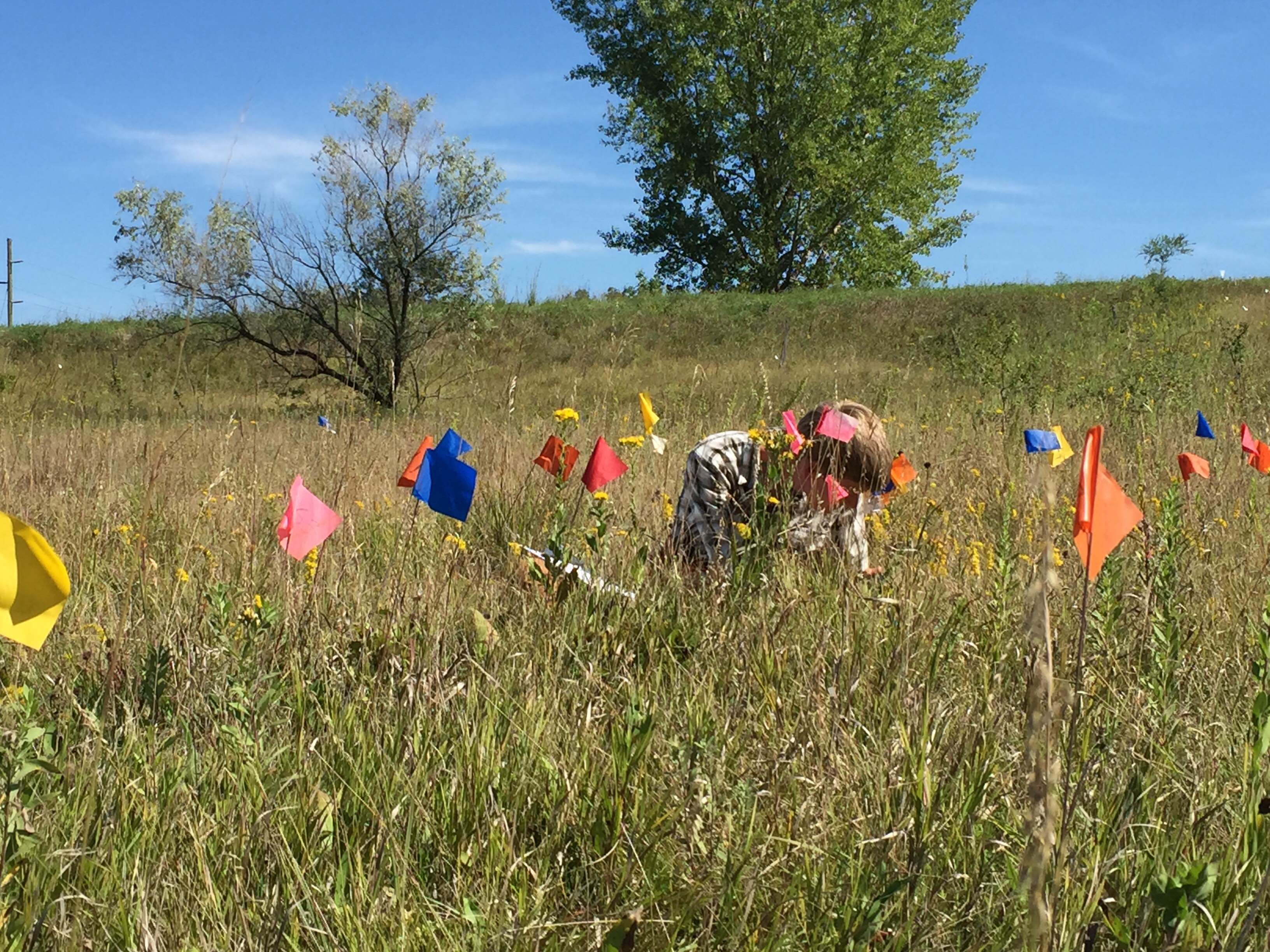
 One of many visits to each flowering plant in prairie remnants. Assessing fitness is a key part of understanding change in any population. The Echinacea Project has focused on two quantifiable components of reproductive fitness of Echinacea angustifolia: style persistence and seed set. Styles shrivel when they receive compatible pollen, and thus persistence of styles reflects pollen limitation. A floret sets a seeds only when it has been successfully pollinated. Together, these two indicators can be used to predict how effectively individual plants produce viable offspring, giving insights into the persistence of remnant populations.
This year, we counted shriveled and non-shriveled rows of styles on each flowering head of every plant in 28 remnants three times per week. Well after the flowering season, we harvested 104 heads at a subset of these sites. The harvested heads will have their achenes removed, counted, and x-rayed by citizen science volunteers to estimate how many seeds they produced. There were several concurrent projects this summer and in the lab that use these measures, including Amy Waananen’s compatibility study and James Eckhardt’s study of edge effects.
Year: 1996
Location: Roadsides, railroads and rights of way, and nature preserves in and near Solem Township, Minnesota.
Overlaps with: flowering phenology in remnants, mating compatability in remnants
Physical specimens: 104 harvested heads, currently at the Chicago Botanic Garden
Data collected:
- Style persistence data for each flowering head, collected three times per week, stored in remData
- Dates and identities of harvested heads, stored on paper datasheets in Harvest 2016 binder and entered electronically into remData
GPS Points Shot: A point for each flowering head, stored under PHEN and SURV records in GeospatialDataBackup
Products:
You can find out more about reproductive fitness in the remnants and read previous flog posts about it on the background page for the experiment.
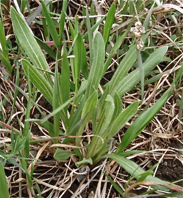
An Echinacea seedling. Between the summers of 2007 and 2013, team Echinacea observed the recruitment of Echinacea angustifolia seedlings around focal plants at 13 different prairie remnants. The locations of these seedlings were mapped relative to each focal plant and the seedlings (now former seedlings) are revisited each year. For each of these former seedlings, we make a record each year updating its status (e.g., basal, not found), rosette count, and leaf lengths. We also try to update the maps, which are kept on paper and passed down through the years, and add toothpicks to note useful landmarks when searching. This summer, we checked 119 focal plants at 12 remnants for 239 former seedlings. We found 148 of these former seedlings (out of the original 955). Although challenging to obtain, this data on the early stages of E. angustifolia in remnants is valuable and rare for us, as nearly all of our data from the remnants comes from plants that have already flowered (several years after first establishing). This data can tell us, for example, how long it takes plants to flower, and the mortality rate among seedlings in remnants.
Year started: 2007
Location: East Elk Lake Road, East Riley, East of Town Hall, KJ’s, Loeffler’s Corner, Landfill, Nessman, Riley, Steven’s Aproach, South of Golf Course remnants and Staffanson Prairie Preserve.
Overlaps with: Demographic census in remnants
Data collected:
- Electronic records of status, leaf measurements, rosette count, and 12-cm neighbors for each seedling. Currently in Pendragon database
- Updated paper maps with status of searched-for plants and helpful landmarks
Products: Amy Dykstra used seedling survival data from 2010 and 2011 to model population growth rates as a part of her dissertation.
You can read more about the seedling establishment experiment and links to previous flog entries about the experiment on the background page for this experiment.
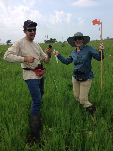
 Alex and Lea measure qGen3 seedlings with much enthusiasm. The main goal of the qGen2 and qGen3 experiments is to quantify the evolutionary potential of two remnant prairie populations of Echinacea angustifolia by estimating the additive genetic variance of fitness. We make estimates for two mating scenarios. The first scenario is an experimental crossing design with all matings among plants from two “core” sites: SPP and LF (core x core). The second design uses sires (pollen donors) from the core and dams from sites peripheral to the core. The crosses performed (core x core, core x periphery) in this experiment will quantify additive genetic variance for fitness in each site and each experimental group. Additionally, we will test for differentiation among families; do progeny from sires differ after accounting for maternal (dam) effects?
In 2016, we found 1724 two year old plants out of the 2581 locations where plants had previously been found for the qGen2 cohort and 644 seedlings in the qGen3 cohort.
Comparing germination between the qGen2 & qGen3 cohorts:
| exp |
approxFullAcheneCt |
totalAcheneCt |
seedlingCt |
germination |
| qGen2 |
6300 |
26144 |
2581 |
41% |
| qGen3 |
6200 |
19777 |
644 |
10% |
Our crossing success, measured by the proportion of full achenes to total achenes crossed, increased in qGen3 (31%) compared to qGen2 (24%). While we planted approximately the same number of full achenes in the qGen2 & qGen3 cohorts, the germination rate was 4 times greater in qGen2 (41%) compared to qGen3 (10%). This difference was likely due to differences in environmental conditions. The Spring of 2016, was quite dry and probably tough on Echinacea seeds and sprouts.
Start year qGen3: 2015
Start year qGen2: 2013
Location: exPt 1 (dams), remnants Landfill and Staffanson (sires), remnants Landfill (core) & around Landfill (peripheral) and remnants Staffanson (core) & railroad crossing sites (peripheral) (grand-dams), exPt 8 (progeny)
Overlaps with: Heritability of fitness–qGen1
Data collected: We used handheld computers to collect data on seedlings and juvenile plants.
You can find more information about Heritability of fitness–qGen2 & qGen3 and links to previous flog posts regarding this experiment at the background page for the experiment.
For the past three years, studying phenology in the remnants has been a major focus of our summer field work. The motivation behind this study is to understand how timing of flowering affects the reproductive opportunity and fitness of individuals in natural populations. Stuart began studying phenology in remnant populations between 1996 and 1999 and several students also studied certain populations in following years. From 2014-2016, we tracked phenology in all of our remnant populations. This year there were 1040 flowering plants (1500 flowering heads).
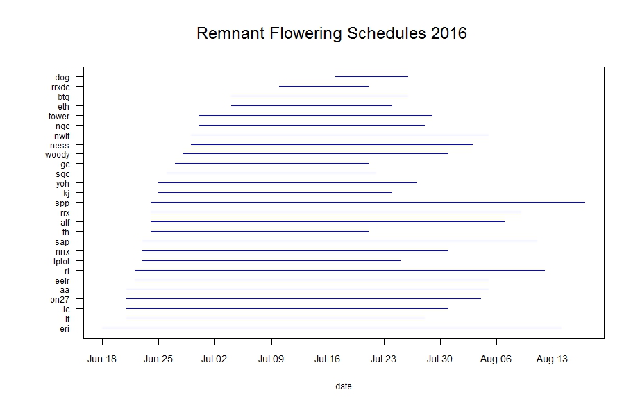
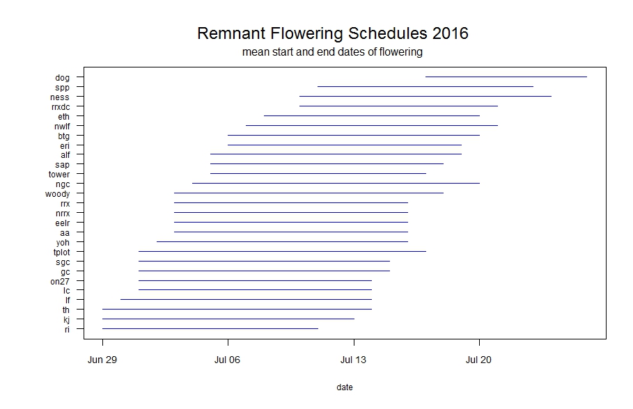
Flowering began on June 18th with one plant at the East Riley roadside remnant. Sadly, this early bloomer was mowed just 6 days after it started flowering. The latest flowering plant shed pollen in the West Unit of Staffanson Prairie Preserve on August 17th. When we consider all populations together, peak flowering was on July 10th. Peak flowering at Staffanson Prairie Preserve was later, on July 18th, likely due to the prescribed burn in the West Unit setting flowering back.
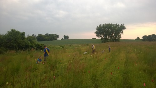
 Line segments represent the duration of flowering for each remnant population. Click to enlarge! As you can see in the figure above, some populations had much longer duration of flowering than others. Flowering duration at Staffanson Prairie Preserve (‘spp’ in the figure) was longer because the west unit was delayed in flowering. East Riley (‘eri’) has a long duration of flowering, likely due to individuals being mowed early in the season, then resprouting and flowering later. This figure shows the very first and last dates of flowering, but population mean start and end dates of flowering is also informative (see what that flowering schedule looks like here). These figure with generated with R package mateable, which was was developed by Team Echinacea to visualize and analyze phenology data.
Start year: 1996
Location: roadsides, railroad rights of way, and nature preserves in and near Solem Township, MN
Overlaps with: Phenology in experimental plots, demography in the remnants
Physical specimens:
- We harvested a random sample of 5 heads from most remnant populations (we excluded very small populations) and brought them back to the lab, where student interns will process and assess their seed set (‘regRem’ or ‘regular remnant harvest’).
- We also harvested the most isolated, least isolated, earliest flowering, and latest flowering individuals from large populations (‘remnant extremes’). Student interns will also process and assess seed set of these heads.
Data collected: We identify each plant with a numbered tag affixed to the stem and give each head a differently colored twist tie, so that each head has a unique tag/twist-tie combination, or “head ID”, under which we store all phenology data. We monitor the flowering status of all flowering plants in the remnants, visiting at least once every three days until all heads were done flowering to obtain start and end dates of flowering. We managed the data in the R project ‘aiisummer2016′ and will add it to the database of previous years’ remnant phenology records.
GPS points shot: We shot GPS points at all of the plants we monitored except for four, two at SGC and two at ERI, which were mowed (ERI) or dug up (SGC) early in the season. These points were shot under job names following the convention “SURV_2016MMDD_SULU” or “SURV_2016MMDD_CHEK”. The locations of plants this year will be aligned with previously recorded locations, and each will be given an identifier (‘AKA’). We will link this year’s phenology and survey records via the headID to AKA table.
You can find more information about phenology in the remnants and links to previous flog posts regarding this experiment at the background page for the experiment.
 We observed that 95% surviving members of the 1996 cohort were basal in 2016 The oldest Echinacea plants in experimental plot 1 are 20 years old. They are part of a cohort planted in 1996 in a common garden experiment designed to study differences in fitness and life history characteristics of remnant populations. Stuart sampled about 650 seeds (achenes) from eight remnant populations in and near Solem Township, representing the range of modern prairie habitat from small patches along roadsides to a large nature preserve. In 1996, he transplanted seedlings on a 1m x 1m grid, randomly assigning the location of each individual.
Every year, members of Team Echinacea assess survival and measure plant growth and fitness traits including plant status (i.e. if it is flowering or basal), plant height, leaf count, and number of flowering heads. We harvest all flowering heads in the fall and obtain their achene count and seed set in the lab.
Only 15 plants from the 1996 cohort were flowering this year. We were very curious to know if this small number was a result of a low rate of flowering or due to high mortality in the cohort. We found that of the original 650 individuals, 291 were alive in 2016, only 13 fewer than last year. That means only 5% of living individuals flowered. In contrast, 45% of living plants flowered last year (and 37% in 2014, 34% in 2013, 40% in 2012). We’re not sure why so few plants flowered this year; it’s possible that individuals flower less as they age, but we also observed low rates of flowering in younger cohorts in experimental plot 1, suggesting that environmental factors may also be responsible.
Start year: 1996
Location: Experimental plot 1
Overlaps with: phenology in experimental plots, qGen3, pollen addition/exclusion
Physical specimens:
- We harvested all 17 heads and at present they await processing at the lab to find their achene count and seed set.
Data collected:
- We used Visors to collect plant growth and fitness traits—plant status, height, leaf count, number of flowering heads, presence of insects—and it has been added to the database (?)
- We used Visors to collect flowering phenology data—start and end date of flowering for all individual heads—which is ready to be added to the exPt1 phenology dataset
- Eventually, we will have achene count and seed set data for all flowering plants (stay tuned)
Products:
You can find more information about the 1996 cohort and links to previous flog posts regarding this experiment at the background page for the experiment.
 Reina, Pamela, and Mike with the photosynthesis machine used in Kittelson et al. (2015) In 2016, we continued the INB2 experiment to investigate the relationship between inbreeding level and fitness in Echinacea angustifolia. Each plant in experiment INB2 originates from one of three cross types, depending on the relatedness of the parents: between maternal half siblings; between plants from the same remnant, but not sharing a maternal or paternal parent; and between individuals from different remnants. We continued to measure fitness and flowering phenology in these plants.
This year, of the original 1,470 plants in INB2, 557 were still alive. Of the plants that were alive this year, 2% were flowering and 75% have never flowered.
Read previous posts about this experiment.
Start year: 2006
Location: Experimental plot 1
Overlaps with: Phenology and fitness in P1, Inbreeding experiment–INB1
Physical specimens: We harvested 9 heads from INB2 that will be processed in the lab with other heads harvested from P1.
Data collected: We used handheld computers to collect fitness data on all plants in INB2.
Products: The below papers were published in summer 2015:
Kittelson, P., S. Wagenius, R. Nielsen, S. Qazi, M. Howe, G. Kiefer, and R. G. Shaw. 2015. Leaf functional traits, herbivory, and genetic diversity in Echinacea: Implications for fragmented populations. Ecology 96:1877–1886. PDF
Shaw, R. G., S. Wagenius and C. J. Geyer. 2015. The susceptibility of Echinacea angustifolia to a specialist aphid: eco-evolutionary perspective on genotypic variation and demographic consequences. Journal of Ecology 103:809-818. PDF
You can find more information about the Inbreeding experiment–INB2 and links to previous flog posts regarding this experiment at the background page for the experiment.
 Reina, Hattie, and Mike with the instrument to measure photosynthesis. In 2016, we continued the INB1 experiment to investigate the relationship between inbreeding level and fitness in Echinacea angustifolia. Each plant in experiment INB1 originates from one of three cross types, depending on the relatedness of the parents: between maternal half siblings; between plants from the same remnant, but not sharing a maternal or paternal parent; and between individuals from different remnants. We continued to measure fitness and flowering phenology in these plants.
This year, of the original 557 plants in INB1, 191 were still alive. Of the plants that were alive this year, 7% were flowering and 24% have never flowered.
Read previous posts about this experiment.
Start year: 2001
Location: Experimental plot 1
Overlaps with: Phenology and fitness in P1
Physical specimens: We harvested 13 heads from INB1 that will be processed in the lab with other heads harvested from P1.
Data collected: We used handheld computers to collect fitness data on all plants in INB1.
Products: The below papers were published in summer 2015:
Kittelson, P., S. Wagenius, R. Nielsen, S. Qazi, M. Howe, G. Kiefer, and R. G. Shaw. 2015. Leaf functional traits, herbivory, and genetic diversity in Echinacea: Implications for fragmented populations. Ecology 96:1877–1886. PDF
Shaw, R. G., S. Wagenius and C. J. Geyer. 2015. The susceptibility of Echinacea angustifolia to a specialist aphid: eco-evolutionary perspective on genotypic variation and demographic consequences. Journal of Ecology 103:809-818. PDF
You can find more information about the Inbreeding experiment–INB1 and links to previous flog posts regarding this experiment at the background page for the experiment.
 Team Echinacea measuring plants in big batch The qGen1 (quantitative genetics) experiment is designed to quantify the heritability of traits in Echinacea angustifolia. We are especially interested in Darwinian fitness. Could fitness be heritable? During the summer of 2002 we crossed plants from the 1996 & 1997 cohorts of exPt1. We harvested heads, dissected achenes, and germinated seeds over the winter. In the Spring of 2003 we planted the resulting 4468 seedlings (this great number gave rise to this experiment’s nickname “big batch”). In 2016 we assessed survival and fitness measures of the qGen1 plants. 2,187 plants in qGen1 were alive in 2016. Of those, 5% flowered in 2016 and 49% have yet to flower.
Start year: 2003
Location: Experimental plot 1
Overlaps with: qGen2 & qGen3
Physical specimens: We harvested 116 heads from qGen1 in 2016. These heads will be processed in the lab to determine achene count and seed set.
Data collected: We collected fitness measures using handheld computers.
Products: We have an awesome dataset that we will share once the paper is published. Ruth Shaw is working on an analysis of the qGen1 dataset.
You can find more information about Heritability of fitness–qGen1 and links to previous flog posts regarding this experiment at the background page for the experiment.
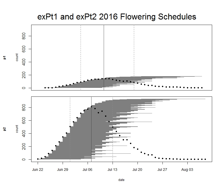
Every year we keep track of flowering phenology in our main experimental plots, exPt1 and exPt2. Fewer plants than usual flowered in exPt1 in 2016: 149 plants (179 heads) flowered between June 24th and August 7th. The population’s mean start date of flowering was July 5th and the mean end date was July 18th. Peak flowering in 2016 was on July 10th, when 143 heads were in flower. For comparison, peak flowering in 2015 was on July 27th, when there were nearly 10x as many heads flowering as on this year’s peak. The earlier phenology and low numbers of flowering we observed this year relative to 2015 is likely due at least in part to the plot burn schedule (2015 was a burn year and 2016 was a non-burn year), but there were still many fewer flowering plants than any season, burn or non-burn, in the past 10 years.
We kept track of 934 flowering heads in ExPt2, where the first head started shedding pollen on June 22 and the latest bloomer ended flowering on August 8th. Peak flowering was on July 7th, when 810 heads were flowering. ExPt2 was designed to study the heritability of phenology—you can read more about progress of that experiment in the upcoming 2016 heritability of phenology project status update.
At the end of the season we harvested the heads and brought them back to the lab, where we will count fruits (achenes) and assess seed set.
 ExPt1 and Expt2 flowering schedules from 2016. Dots represent the number of flowering heads on each date. Horizontal line segments represent the duration of each heads flowering and are ordered by start date. The solid vertical line indicates peak flowering, while the dashed lines indicate the dates when 25% and 75% of heads had begun flowering, respectively. Click to enlarge! Start year: 2005
Location: Experimental Plots 1 and 2
Overlaps with: Heritability of flowering time, common garden experiment, phenology in the remnants
Physical specimens: We harvested 177 heads from exPt1 and 870 from exPt2. Attentive readers may note that we harvested about 64 fewer heads than we tracked for phenology. That’s because before we could harvest many seedheads at exPt2, rodents chewed through their stems and ate some fruits (achenes). We recovered most of the heads that were grazed from the ground and made estimates of number of fruits lost due to herbivory, but we couldn’t find some heads. Arg. We brought the harvest back to the lab, where we will count fruits and assess seed set.
Data collected: We visit all plants with flowering heads every three days until they are done flowering to record start and end dates of flowering for all heads. We managed phenology data in R and added it to the full dataset. The figure above was generated using package mateable in R. If you want to make figures like this one, download package mateable from CRAN!
You can find more information about phenology in experimental plots and links to previous flog posts regarding this experiment at the background page for the experiment.
 We revisited locations in remnants where flowering plants were observed in previous years. We tag each Echinacea plant we see flowering in our prairie remnants, and record its location using the GPS. This is useful because it allows us to revisit the same plant in future years, checking to see if it is still alive, and if so how large it is and whether or not it is flowering. This has provided us with a very rich longitudinal dataset of life histories, dating back two decades and including thousands of plants. This year, we did total demo, visiting each plant in our database, at several sites including Staffanson, Loeffler’s Corner East, Northwest of Landfill, and East Elk Lake Road. In the interest of time, we only did flowering demo (only visiting plants that flowered this year) at several sites, including Landfill, Around Landfill, and Railroad Crossing. For each plant visited, we recorded its status (e.g., basal, flowering), its number of rosettes, and any neighboring Echinacea within a 12 cm radius. This data can be used to study inter-annual variation in flowering, population dynamics, and response to fire.
Year: 1996
Location: Roadsides, railroad rights of way, and nature preserves in and near Solem Township, Minnesota.
Overlaps with: Flowering phenology in remnants, fire and flowering at SPP
Data collected: Flowering status, number of rosettes, number of heads, neighbors within a 12 cm radius of plants found, stored in demo2016
GPS points shot: Points for each flowering plant this year shot mostly in PHEN records, stored in surv.csv. Some points of flowering plants stored in SURV records, also in surv.csv. Each location should be either associated with a loc from prior years or a point shot this year.
Products:
- Amy Dykstra’s dissertation included matrix projection modeling using demographic data
- Project “demap” merges phenological, spatial and demographic data for remnant plants
You can find out more about the demographic census in the remnants and links to previous posts regarding it on the background page for this experiment.
|
|

