|
|
With all of my data collected and visualized for the heads from Staffanson Prairie Preserve from 2015, it is now time to start with some initial data analysis. As I mentioned in my last post, I will be using R for all of my analyses, taking advantage of skills I learned in Stuart’s class at Northwestern this quarter. I will be creating statistical models based on the data to look for relationships between variables that may influence mate availability and reproductive success. The variables I am specifically looking at are:
- Distance to the kth nearest flowering neighbor. This is a measure of spatial isolation, with greater distance indicating greater isolation. Stuart has found a significant relationship between distance and reproductive success in Echinacea previously (that study can be found here: https://echinaceaproject.org/pub/wagenius2006.pdf)
- Start date and flowering duration. Flowering phenology, the timing and duration of flowering, is perhaps more important than spatial isolation in determining availability of compatible mates. If two plants are very close in space, but they do not flower at the same time, there is no possibility for mating. Previous data has shown that plants flowering earlier in the season have higher reproductive success (https://echinaceaproject.org/pub/isonAndWagenius2014.pdf)
- Section of head from which the achene originated. Because florets at the base Echinacea heads begin flowering first, and the ones at the top flower last, it is possible to examine how reproductive success, and thus the mating scene, differ for a single head across time. The bottom 30 achenes, the middle achenes, and the top 30 achenes are separated to represent the beginning, middle, and end of the timing of flowering.
- Seed set, or proportion of achenes that contain a seed, will be used to quantify reproductive success. This will be the that the model I create will try to predict using the variables I listed above.
In order to create a model, I will be using a technique known as backwards elimination as described in Statistics: An Introduction Using R (Crawley 2015). I will start by creating a statistical model containing my response variable (seed set), and all of my explanatory or predictive variables (isolation, phenology, section of head), along with all interactive effects between the explanatory variables. I will then eliminate a single predictor or interaction at a time and perform an analysis of deviance to determine whether or not that predictor was important to the predictive value of the model. If it is important, I will leave it in, but if it’s not, I will take it out. This process continues until all predictors and interactions left in the model have a significant effect on the response. This model, known as the minimal adequate model, is the simplest model that still includes all important variables.
Now that I’ve finished collecting data from the Echinacea heads collected from Staffanson Prairie Preserve in 2015, I am able to start doing some data analysis. While the ultimate goal is to compare the data from 2015, a non-burn year, to previous burn years, I first want to come to a good understanding of what reproductive success looked like in 2015.
For all of the analyses I will be doing, I am using computer software called R. R is a very flexible program that allows you to employ a wide range of graphical and statistical techniques including modeling, running tests, and clustering. Although R does have a somewhat steep learning curve, I have been learning many useful techniques in Stuart’s class on R at Northwestern and am confident in my ability to properly analyze the data I have collected.
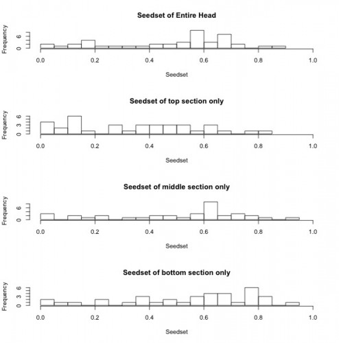
The histograms below show seedset, which is the proportion of achenes that contain a seed and can range from zero to one, for the entire head, as well as for the top, middle, and bottom sections of each head. For the entire head, the sample has a range from 0 to 0.86, with a mean of 0.48 and a median of 0.57. While the middle and bottom portions of the head had similar seedsets, the top portions of each head appear to have lower seed set on average when compared to the rest of the head. This is consistent with the findings of previous years and suggests that florets that are receptive to pollen later in the season may have diminished reproductive success.

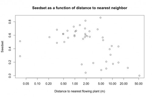
An important variable in Echinacea reproduction, spatial isolation, is modeled in the below plot as a predictor of seedset. This plot highlights the importance of doing a careful visual exploratory data analysis before diving into more complicated statistical analyses. While there does appear to be the expected inverse relationship between seedset and spatial isolation, upon looking at this plot Stuart was immediately able to tell me that the two points on the left of the plot are the result of erroneous data. None of the plants have a nearest neighbor less than 5 cm away, so there must have been an error either in data entry or during the recording of GPS coordinates. Because we have records for the correct GPS coordinates of every plant, this will be a very easy error to fix, but had Stuart not looked closely at this plot, I may have done the entire analysis with incorrect data.

Much of the work I have been doing up to this point has been to determine a single number for each head—the proportion of all achenes on a given head that contain a fully formed seed, or seed set. This gives a good indication of how successful that plant was in terms of reproduction. The most likely reason that an achene does not contain a seed is that the flower did not receive compatible pollen, either due to a lack of mates or due to a limitation on the part of the pollinators.
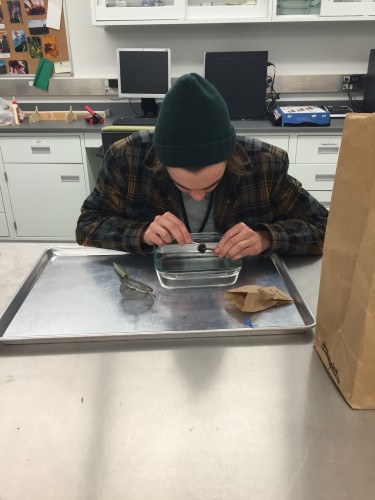
In order to determine seed set, I need two numbers: the total number of achenes and the number of achenes containing an embryo. While the achenes could be counted by hand, this would be a tedious and error-prone process. Instead, the achenes were placed on a glass tray and scanned into the computer and counted digitally.
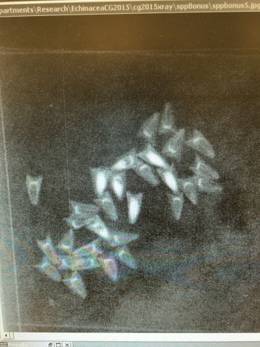
It is possible to determine whether or not an achene contains a seed by several methods. Germination experiments are useful because every achene that germinated certainly contained a seed, but they can be time-consuming and demand lots of attention and resources. Another possibility is to weigh the achenes. Heavier achenes are much more likely to contain a seed, and lighter achenes are most likely empty. We chose to use x-ray, which allows us to see directly inside of each achene. When achenes are x-rayed, empty achenes are barely visible while seeds show up as opaque. Ideally, all achenes could be easily categorized into “empty” or “full,” but some achenes are partially full, likely meaning they were initially fertilized but full seed growth was not entirely successful.
Together, these numbers are very important in allowing us to make inferences about what conditions are best for Echinacea reproduction.
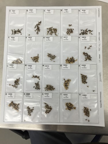
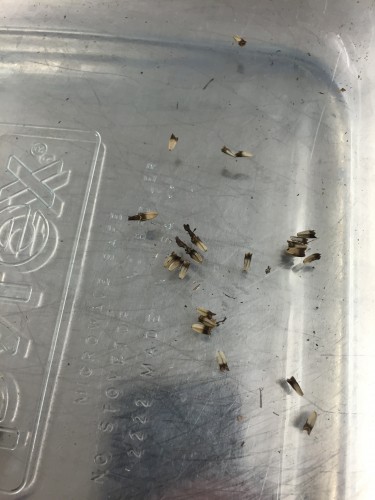
 Randomized achenes ready to be x-rayed.
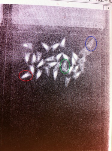
This is what x-rayed achenes look like. Achenes that contain a seed show up with a white oval in the center.  Full, partial, and empty achenes are counted on the computer and entered into an spreadsheet.
Randomization is a critical aspect of any experiment. In almost all cases, the population being studied is much too large to study every individual, so a sample of the population is studied with the assumption that trends and relationships seen in the sample are also present in the population as a whole. In order for this to be a good assumption, the sample must be completely random in order to eliminate any bias towards a specific type of individual.
In an ideal world, all samples would be completely random, but this is not logistically possible in many cases. For example, at Staffanson Prairie Preserve, there are thousands of Echinacea that bloom every year. It would be a near impossibility to visit every single plant or even to select a completely random sample of plants within the preserve. For this reason, the Echinacea Project created a 10-meter wide transect through the preserve and studies the plants that fall within this transect. While this is not a truly random sample, it is able to approximate the range of conditions seen throughout the preserve.
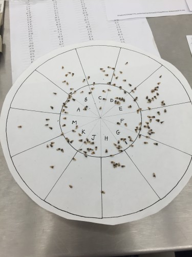
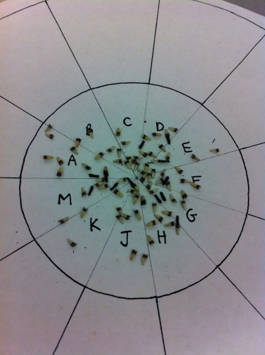
Another example of randomization is something I’ve been working on in the lab for the last week. Many of the heads contain several hundred achenes, so x-raying all of them to determine whether or not they contain a seed would be extremely time consuming and difficult. In order to simplify the process, I am randomly selecting 1/6th of the achenes from each head in order to estimate seed set for each head. While this will not give me the exact seed set, it will give me a very good approximation that will be sufficient for our analyses. Pictures of the randomization process are shown below—achenes are randomly dispersed on a wheel divided into twelve labeled sections of equal size. Next, two letters are selected from a list of random letters, and the achenes that fall within these sections are selected to be x-rayed.
Achenes on the randomization wheel Randomized achenes–labeled and ready for x-raying
For the past three weeks, I’ve been hard at work collecting the achenes from Echinacea heads that were collected last summer from Staffanson Prairie Preserve. A little bit of Echinacea anatomy to give you a better idea of what I’m talking about: each head typically consists of 100 to several hundred small flowers or florets. After the head has matured and the florets have finished blooming, every flower produces one fruit, known as an achene, regardless of whether or not it was fertilized. Back at the lab, we clean all the achenes off the heads in order to count them and determine whether or not they contain a viable seed.
An intact head Achenes In addition to cleaning the heads, I have also been separating the achenes by where on the head they were located. The florets bloom row-by-row starting from the base of the head and working their way up, so we know that the florets at the bottom bloomed first and the ones at the top bloomed last. Looking at reproductive success via seed set on the top, middle, or bottom of each head will thus give an indication of how the mating scene and pollen availability changed over the course of the mating season.
Hard at work cleaning a head Cleaning the heads is the first step in determining seed set, the primary measure of reproductive success I’ll be using for this project. Seed set is defined as the proportion of seeds that were successfully fertilized, and this number can range from zero to nearly 100%. While there are many reasons that fertilization may have failed, the primary reason is most likely a lack of compatible pollen. Now that all the achenes have been removed from the heads, I can determine what proportion of achenes on each head contains an embryo using x-ray. I’ll go into more depth about the x-raying process in another post.
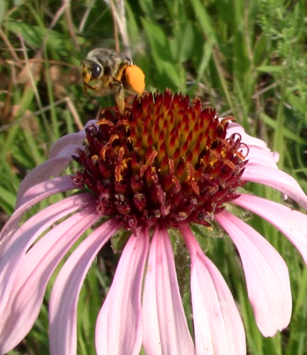
What an incredible three weeks! I wouldn’t have bee-lieved you if you told me three weeks ago everything I would learn! I would have said “quit pollen my leg”. On my first day working at the Chicago Botanic Garden I didn’t know a thing about native bees. Now, I have learned all about the bees that visit Echinacea, from their size to their nesting habits to fun facts about pollen regurgitation and flight velocity. I learned how to navigate DiscoverLife and how to examine a specimen under the microscope, looking for all the little distinguishing traits that make each species special, from the color on the tips of their mandibles to the distance from the rim the hair band on the T4 section of the abdomen rests. The collection of over 900 specimen is now all neatly organized and a reference collection is all packed and waiting to be used in the field this summer. The Echinacea Project youtube account is now set up and loaded with videos of all these little pollinators visiting Echinacea and working their hardest. And, finally, the database on the Echinacea webpage is complete, filled with links and beautiful pictures galore, ready to be poured over by future bee-lovers and scientists alike in the quest to explore the worlds of these bee-utiful pollinators! I want to thank the team here so much for your kindness and for all of your help along the way. Hive-five, everyone!
Happy Wednesday, readers! It’s hard to believe that this will be our last Wednesday here at the Garden, but it is—things are winding down. Well, sort of winding down. We still have a lot of work to do! For me and Jackie, we’ve finally gotten to start the data analysis (also known as the fun part).
But first, we had to do all of the x-raying! We mentioned it briefly in some other posts, but here’s what the results actually ended up looking like:

We then had to look through the images and count which achenes were full, empty, or partially-full (shown in red, blue, and green, respectively). We use these x-rays to get a sense of seed-set, or how well the Echinacea heads were fertilized. All of the previous steps have been looking at achenes, which are actually the fruit of the flower. All the heads produce achenes, but only some of those achenes have seeds that will grow into more Echinacea. In this way, the x-raying can be considered the most important part; it’s measuring reproduction most directly. Also interesting to note: the x-raying protocol is very careful to minimize the x-ray exposure of achenes being studied. That way, any seeds produced are more likely to be viable, and still grow later!
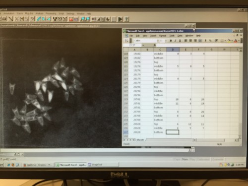
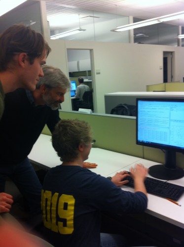
With that out of the way, we’re on to the fun of analysis, which doesn’t actually look that fun (unless you like computers):

Whoops, I accidentally got my finger in the shot.
We’ll be spending a lot of time manipulating our data in R (as shown) and feeding it into models. The idea is to test whether achene location on the head, plant isolation, and flowering timing relate to seed-set. Tune in on Friday for results!
If you have been obsessively checking the Echinacea Project website every few minutes today (as I often do), you will probably have noticed we have added an addition to our beautiful home! After many hours of crashing, banging, hammering, crying, and all those fun things that come with construction and home renovation, we now have a bee field guide. Take the time to explore it, but explore with great caution, as I am positive there are still bugs (hehe) to be fixed. Over the next few days I will right the wrongs and tie up all the loose ends.
What pun should I end with? Perhaps I will continue the metaphor- back to the buzzing of the drill!
We thought the worst was behind us- that all the heads had been cleaned. Today, we found out we were wrong. After digging up (literally) the remaining heads to be cleaned, cleaning, scanning, counting, and randomizing them, it seems like all that’s left is some x-raying and our data set will be complete.
That is, we would be done, if at the end of the day we hadn’t finally found the very last uncleaned head. It had been filed away a little precariously, but no matter. We look forward to tomorrow, when we will have hopefully finished most of the data collection, and can start into our analysis.
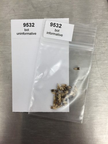
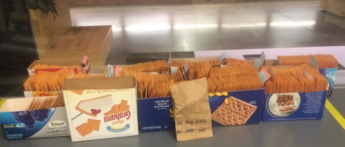
See Below- the impressive (to me, anyway) quantity of coin envelopes we’ve filled with seeds from different sections (top, middle, bottom) of each head, and (officially) the very last head to be cleaned.

With our second of three weeks coming to a close, the externs are working hard to get their projects finished. While Belle is still busy with the pollinator database, Audrey and Jackie have been desperately trying to finish processing all the randomly sampled heads from the remnant prairie populations. This processing isn’t quick–that’s why it’s taken up the majority of our externship. As mentioned previously, processing has five steps: cleaning or dissecting the head to get all the achenes out, scanning the achenes, counting the achenes, randomizing a sample of the achenes to x-ray, and finally x-raying the achenes for the presence of seeds. Now that we’re finally done with all of the cleaning, we’ve been focusing on scanning, counting, and randomizing so that we can get x-raying next week. Here’s a behind-the-scenes look at how we’ve been doing these steps:
The scanning is just how it sounds: we very carefully pour the achenes out onto a standard office scanner and get an image of them. This image is what we use for counting. It may seem superfluous to scan the achenes and count from the image when we could count the achenes themselves, but when heads often have more than 200 achenes, it’s tough to accurately count by hand. Computers are much better of keeping track of what number they’re on, so we let them do the work. Once the image is scanned, we just have to click on each achene we see in the image and it’s marked with a dot. The computer keeps track of the number of dots. That way, you know you haven’t missed any achenes and that your number is accurate. Here’s Jackie, in action counting:
After scanning, I’ve been taking the achenes and randomizing them. In other words, I’ve been taking all the achenes from the middle of the head and taken a random sample of 1/6 of all the middle achenes. This is done pretty simply: you take the achenes and pour them out onto a circle divided into wedges and labeled with letters. Then, from a list random letters, you determine which wedges you’re taking achenes from. For the picture below, for example, the achenes chosen for x-raying were from wedges G and H:
If you think these steps sound a little tedious, you’re right. But, we’re hoping all this processing leads to some really interesting data to analyze next week!
|
|