|
|
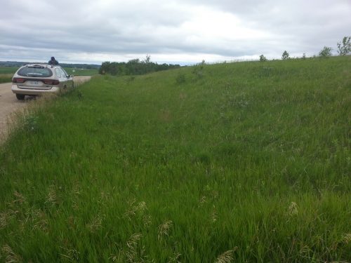
All the first year researchers were assigned a study site to visit and observe. East Elk Lake Road, located in the northwest corner of the study area, is a small reserve that has not been actively maintained. The site lies just off a gravel road and consists of plants by the roadside, with a ditch and hillock that run for around 200 meters alongside the road. A wetland surrounded by trees lies at the western edge of the study site, and the trees are encroaching on the prairie fragment. The study site is across the road from a larger prairie fragment contributing to a larger gene pool. The site south of the road had similar plant diversity suggesting more active management.
This study site was characterized by three different sets of plants. The edge of the gravel road is disturbed and the flora consists of a high abundance of brome as well as dandelion and Poa. Just beyond the disturbed road edge is a shallow ditch and sloping hillside. This area contained the highest diversity of forbs, grasses and legumes, many of which are native. Grasses included big bluestem and needle and thread grass. There were many native forbs, including Canada anemone, goldenrod and bedstraw. This was the only area in which Echinacea (a clump of four individuals) was found. We also found asparagus plants, some of which looked ready to eat! While many legumes are found in most study sites, this site had a surprising few native and nonnative legumes. Leadplant also grew along the hillside. The top of the hillock was densely covered in nonnative brome, along with some relatively dense dogbane and prairie rose, but this area showed lower diversity than the hillside. This summit also featured tree saplings, no higher than five feet tall.
The size of woody trees and shrubs in the area and the large amount of duff on the hilltop suggests the site had not been burned for many years. Plant cover on the hilltop as well as an overgrown access road (we call this an approach) to the hilltop suggested the area had been used for grazing or farm fields.
 View West from approach with brome along the gravel road shown on the left
Echinacea Project 2016
Hi everyone! My name is Rachel Rausch, and I’m so excited to be a part of Team Echinacea this summer. I graduated from Morris Area High School a few weeks ago, and will be attending the University of Minnesota Twin Cities this fall, studying Psychology.
Research Interests
Because UMN is a research institution, I’m looking forward to getting research experience this summer. This will be my first hands on experience with conservation biology and I’m excited to learn about the research process.
Statement
I’m from Morris, MN which is about 30 miles from Kensington. I In my free time, I love to read, rollerblade, and enjoy Minnesota’s 10,000 lakes. I love learning new things, and in my 18 years on earth have attempted to knit, play piano, weld, unicycle, and make an ice sculpture.
My name is Chris Woolridge and I’m very excited to begin as a Seasonal Researcher with the Echinacea Project this summer! I’ll be helping Danny and the citizen scientists in the lab while the rest of the team is in Minnesota conducting field work. I’m currently a graduate student in the Plant Biology and Conservation Program at the Chicago Botanic Garden and Northwestern University. My research is focused on better informing seed sourcing for restorations. Some researchers and managers have proposed sourcing seed from more southern latitudes to foster populations that are pre-adapted to climate change. In order to test this strategy’s feasibility, I’m conducting a common garden experiment in Grayslake, IL, investigating relative fitness of plants sourced across a latitudinal gradient in five savanna/prairie species used in restorations. With that being said, I’m very interested in the questions the Echinacea Project is asking and I’m thrilled to be joining the team!

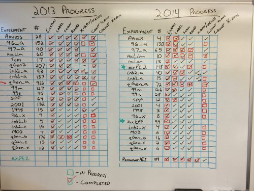
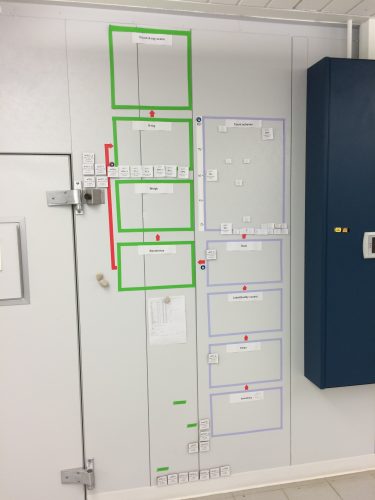
Though Stuart, Gretel, and Amy will be headed to Minnesota for the summer, our wonderful team of volunteers will still be here in Illinois working hard. We’ve used a couple systems to measure progress in the past few years but we’re going to make a simplified version for the summer before completely redoing our lab workflow visualization. We wanted to give our progress boards a proper send off before replacing them with a simpler summer-oriented progress board. More details to come!
 The progress board before being erased.  The progress wall before tape removal
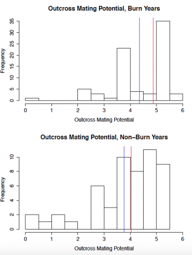
For the past several weeks, I have been busily going through tons of data from previous years in an effort to isolate only the data I need for my project. As a reminder, I’m looking at how prairie fire changes the mating scene and mate availability for Echinacea. I am using data from 1996, 1998, 2007, 2009, 2012, 2014, and 2015. With the exception of 2015 when no burn occurred, part of Staffanson Prairie Preserve underwent a controlled burn during each of these years.
From a file containing all seed set data for all plants that the Echinacea Project has ever collected, I extracted data for plants that flowered in both 2015 and at least one of the previous burn years. I ended up with 26 plants that met this description, and I will compare reproductive success of each of these plants on an individual basis in burn years compared to non-burn years.
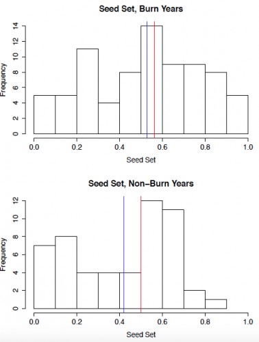
To start out, I created some histograms of the data to get a quick insight into patterns that might be present. In order to roughly quantify the quality of the mating scene for a given plant, I calculated outcross mating potential (OMP), which takes into account the distances to the 6 nearest flowering neighbors. A higher value indicates a greater density of available mates. The second set of histograms shows seed set, with a higher number indicating greater reproductive success. While I will need to conduct statistical analyses to get a better understanding of what these data mean, initial impressions indicate that both the mating scene and reproductive success may be better in burn years.
 
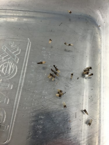
For the past three weeks, I’ve been hard at work collecting the achenes from Echinacea heads that were collected last summer from Staffanson Prairie Preserve. A little bit of Echinacea anatomy to give you a better idea of what I’m talking about: each head typically consists of 100 to several hundred small flowers or florets. After the head has matured and the florets have finished blooming, every flower produces one fruit, known as an achene, regardless of whether or not it was fertilized. Back at the lab, we clean all the achenes off the heads in order to count them and determine whether or not they contain a viable seed.
 An intact head  Achenes In addition to cleaning the heads, I have also been separating the achenes by where on the head they were located. The florets bloom row-by-row starting from the base of the head and working their way up, so we know that the florets at the bottom bloomed first and the ones at the top bloomed last. Looking at reproductive success via seed set on the top, middle, or bottom of each head will thus give an indication of how the mating scene and pollen availability changed over the course of the mating season.
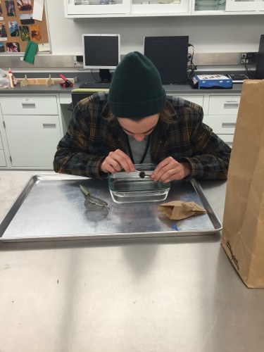
 Hard at work cleaning a head Cleaning the heads is the first step in determining seed set, the primary measure of reproductive success I’ll be using for this project. Seed set is defined as the proportion of seeds that were successfully fertilized, and this number can range from zero to nearly 100%. While there are many reasons that fertilization may have failed, the primary reason is most likely a lack of compatible pollen. Now that all the achenes have been removed from the heads, I can determine what proportion of achenes on each head contains an embryo using x-ray. I’ll go into more depth about the x-raying process in another post.
Happy Wednesday, readers! It’s hard to believe that this will be our last Wednesday here at the Garden, but it is—things are winding down. Well, sort of winding down. We still have a lot of work to do! For me and Jackie, we’ve finally gotten to start the data analysis (also known as the fun part).
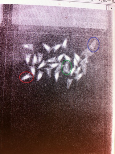
But first, we had to do all of the x-raying! We mentioned it briefly in some other posts, but here’s what the results actually ended up looking like:

We then had to look through the images and count which achenes were full, empty, or partially-full (shown in red, blue, and green, respectively). We use these x-rays to get a sense of seed-set, or how well the Echinacea heads were fertilized. All of the previous steps have been looking at achenes, which are actually the fruit of the flower. All the heads produce achenes, but only some of those achenes have seeds that will grow into more Echinacea. In this way, the x-raying can be considered the most important part; it’s measuring reproduction most directly. Also interesting to note: the x-raying protocol is very careful to minimize the x-ray exposure of achenes being studied. That way, any seeds produced are more likely to be viable, and still grow later!
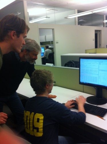
With that out of the way, we’re on to the fun of analysis, which doesn’t actually look that fun (unless you like computers):

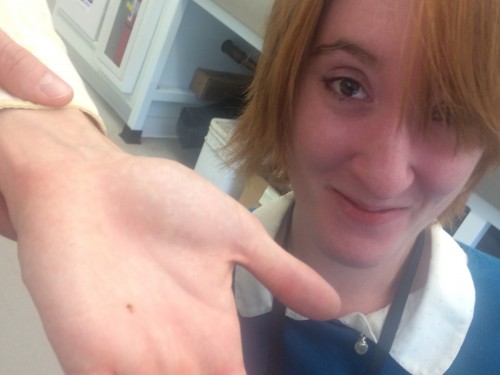
Whoops, I accidentally got my finger in the shot.
We’ll be spending a lot of time manipulating our data in R (as shown) and feeding it into models. The idea is to test whether achene location on the head, plant isolation, and flowering timing relate to seed-set. Tune in on Friday for results!
With our second of three weeks coming to a close, the externs are working hard to get their projects finished. While Belle is still busy with the pollinator database, Audrey and Jackie have been desperately trying to finish processing all the randomly sampled heads from the remnant prairie populations. This processing isn’t quick–that’s why it’s taken up the majority of our externship. As mentioned previously, processing has five steps: cleaning or dissecting the head to get all the achenes out, scanning the achenes, counting the achenes, randomizing a sample of the achenes to x-ray, and finally x-raying the achenes for the presence of seeds. Now that we’re finally done with all of the cleaning, we’ve been focusing on scanning, counting, and randomizing so that we can get x-raying next week. Here’s a behind-the-scenes look at how we’ve been doing these steps:
The scanning is just how it sounds: we very carefully pour the achenes out onto a standard office scanner and get an image of them. This image is what we use for counting. It may seem superfluous to scan the achenes and count from the image when we could count the achenes themselves, but when heads often have more than 200 achenes, it’s tough to accurately count by hand. Computers are much better of keeping track of what number they’re on, so we let them do the work. Once the image is scanned, we just have to click on each achene we see in the image and it’s marked with a dot. The computer keeps track of the number of dots. That way, you know you haven’t missed any achenes and that your number is accurate. Here’s Jackie, in action counting:

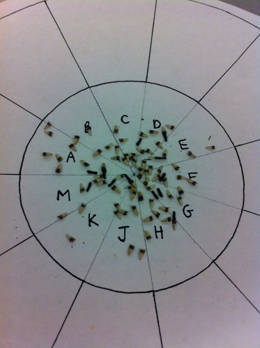
After scanning, I’ve been taking the achenes and randomizing them. In other words, I’ve been taking all the achenes from the middle of the head and taken a random sample of 1/6 of all the middle achenes. This is done pretty simply: you take the achenes and pour them out onto a circle divided into wedges and labeled with letters. Then, from a list random letters, you determine which wedges you’re taking achenes from. For the picture below, for example, the achenes chosen for x-raying were from wedges G and H:

If you think these steps sound a little tedious, you’re right. But, we’re hoping all this processing leads to some really interesting data to analyze next week!
Today we kicked off week two of three of our externship. After a restful weekend checking out downtown Chicago, everyone’s back to work on their respective projects. While Belle’s been busily researching the lab’s collection of bees, Jackie and Audrey have been hard at work trying to process all of our remnant seed heads so we can do some data analysis. It turns out we have a lot more heads to process than we thought! With the entire process—cleaning the heads, scanning them, counting the number of achenes, randomizing samples for x-raying, and x-raying for the presence of seeds– each head takes a long time to get completely ready. So, we’ve decided to scale back our analysis to just randomly selected flowers for now, instead of looking at a random sample as well as heads with extremes of early and late flowering times. Audrey’s been busy trying to get all the scanned heads ready for x-raying, so lots of selecting random samples and labeling of clear plastic bags. Jackie’s been busy cleaning—even testing out the Optivisor to see if magnifying the heads speeds things up:

We’ve also found four more larval friends! We’ve gotten around 10, now.
Halfway through our first week of the externship, things have started getting exciting! While Belle has been busy cataloguing, Jackie and Audrey have made some new friends: larvae we’ve found living in the seed heads. The mystery larvae are unfortunately eating the achenes we’re trying to collect, but to make the most out of a bad situation, we’ve been collecting larvae, too! The count in our petri dish is about 8, and growing! Most of these have been found by Audrey, who in a twist of cruel irony is the most startled to find them. The larvae are pretty big relative to the head and easy to spot (they’re pale pink and the heads are dark brown), but we still haven’t figured out how to predict which achene we pull out will have a larva behind it. We still have a lot more heads to clean and find larvae in, so we hope to find out where they’re coming from and maybe even see what they turn into.
Pictured below: Jackie and Audrey’s first larval finds.
 
|
|
