This summer Team Echinacea did demo and surv in 42 prairie remnants and other sites with Echinacea angustifolia populations. Demo involved measuring traits of individual plants: flowering status, number of flowering heads, and near neighbors. This summer we took 5119 demo records on our handheld data collectors (visors). Surv involved tagging individual plants and recording their location with our super-precise GPS (Darwin). This summer we shot 1494 points for surv. For ‘total demo’, we navigated to adult Echinacea plants that have been previously visited and took demo to generate detailed, long-term records of individual fitness in these fragmented Echinacea populations. At smaller sites we collected data on all adult plants and at larger sites we visited a subset of the adult plants. The demo and survey datasets are in the process of being combined with previous years’ records of flowering plants in “demap,” the spatial dataset of remnant reproductive fitness that the Echinacea Project maintains.
Start year: 1995
Location: Remnant prairie populations of the purple coneflower, Echinacea angustifolia, in Douglas County, MN. Sites are located between roadsides and fields, in railroad margins, on private land, and in protected natural areas.
Total demo: Bill Thom’s Gate, Common Garden, Dog, East of Town Hall, Golf Course, Hegg Lake, Martinson’s Approach, Nessman, North of Golf Course, REL, RHE, RHP, RHS, RHX, RKE, RKW, Randt, Railroad Crossing Douglas County, South of Golf Course, Sign, Town Hall, Tower, Transplant Plot, West of Aanenson, Woody’s, Yellow Orchid Hill
Annual sample: Aanenson, Around Landfill, East Elk Lake Road, East Riley, KJ’s, Krusemarks, Loeffler’s Corner, Landfill, North of Railroad Crossing, Northwest of Landfill and North of Northwest of Landfill (lumped), On 27, Riley, Railroad Crossing, Steven’s Approach, Staffanson Prairie
Data: Dropbox/geospatialDataBackup2020 contains the experiment’s GPS files and the aiisummer2020 repo contains its demo records. The most recent copies of allDemoDemo.RData and allSurv.RData are accessed at Dropbox/demapSupplements/demapInputFiles.
Products: Amy Dykstra’s dissertation included matrix projection modeling using demographic data. The “demap” project merges phenological, spatial and demographic data for remnant plants.
For more information on demographic census in the remnants, visit the experiment’s background page, or explore flog entries that mention the experiment.
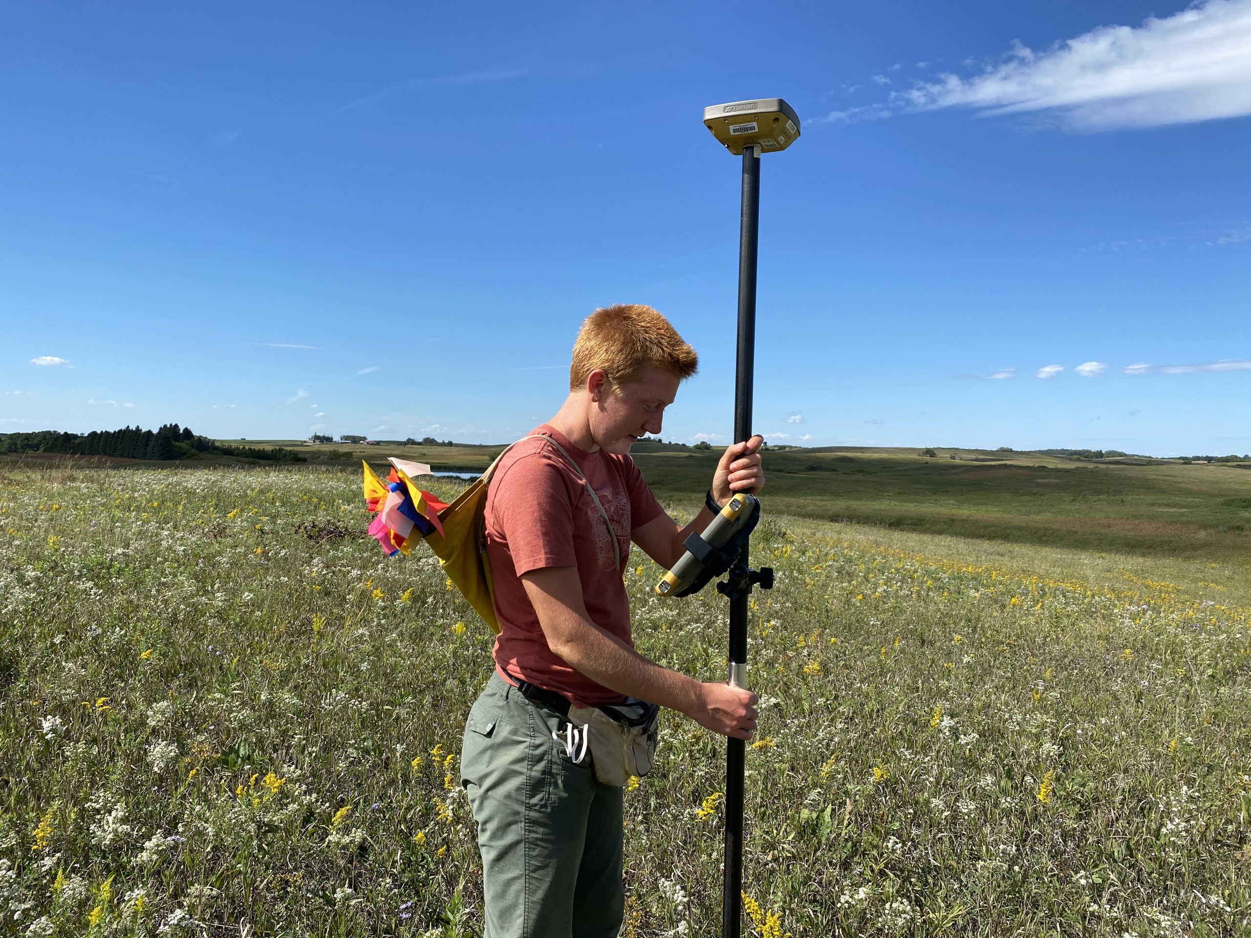
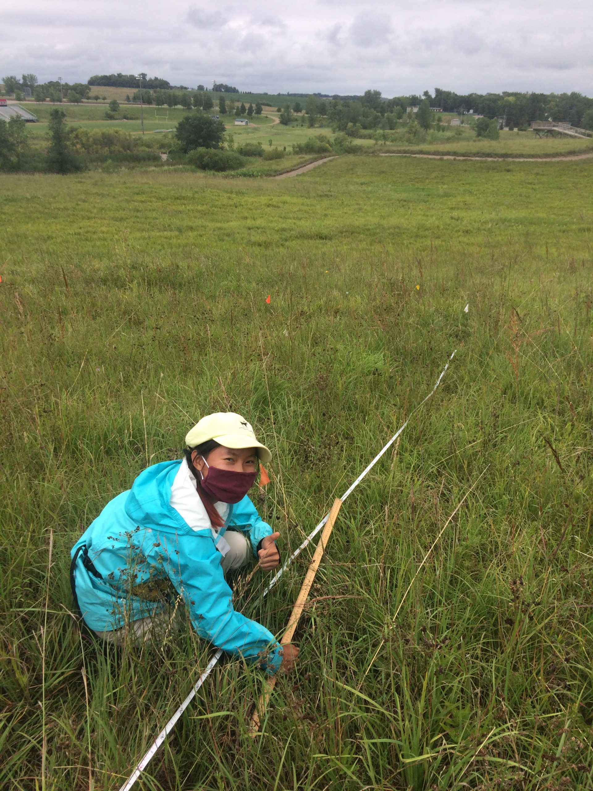
Emma using Darwin, our survey-grade GPS, in late August near Hegg Lake
Monitoring reproductive fitness in the remnant populations is a staple Team Echinacea summer activity. Understanding the reproductive success of plants in remnant populations provides insight to a vital demographic rate contributing to the persistence (or decline) of remnant populations in fragmented environments.
In the summer of 2020, we harvested 304 seeds heads from 29 populations (AAN, AAS, ALF-E, ALF-W, BTG, DOG, EELR, ERI, ETH, GC, LCE, LCW, NESS, NNWLF, NRRX, NWLF, ON27, RIN, RIS, RRX, SAP, SGC, TH, TOWER, WAA, YOH). These are the same populations where we measured flowering phenology. We randomly selected 15 heads from each population, if a population did not have 15 heads, we harvested all of the heads. We harvested heads from the following populations.
These heads are currently in the CBG lab and soon we will start the process of removing the achenes and assessing seed set. We are unsure how exactly we will assess seed set because the x-ray at the Chicago Botanic Garden isn’t working now. We may weigh the seeds.
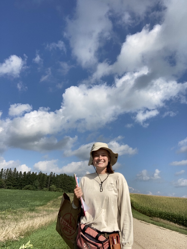
Mia Stevens heading out to harvest
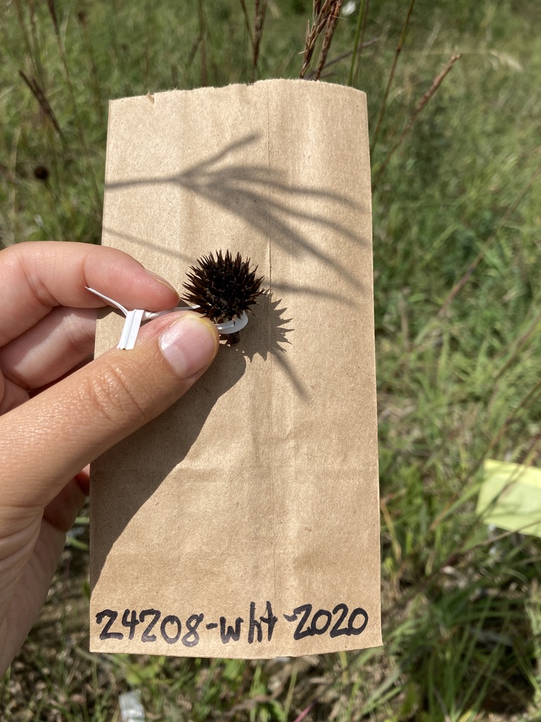
A harvested head
In the spring, we plan on burning some of these remnants and also collecting heads next fall. Estimates of seed set from these heads will serve as a baseline for comparing seed set before and after a burn. We will learn how fire affects reproductive success in small prairie remnants.
Start year: 1996
Location: Roadsides, railroad rights of way, and nature preserves in and around Solem Township, MN
Data/Materials collected: 304 seed heads were collected, these are currently at The Chicago Botanic Garden along with the paper data sheets. These data sheets need to be scanned, double-entered, and checked.
Products: We will compile seed set data from 2020 into a dataset with seed set data from previous years.
You can read more about reproductive fitness in remnants, as well as links to previous flog entries mentioning the experiment, on the background page for this experiment.
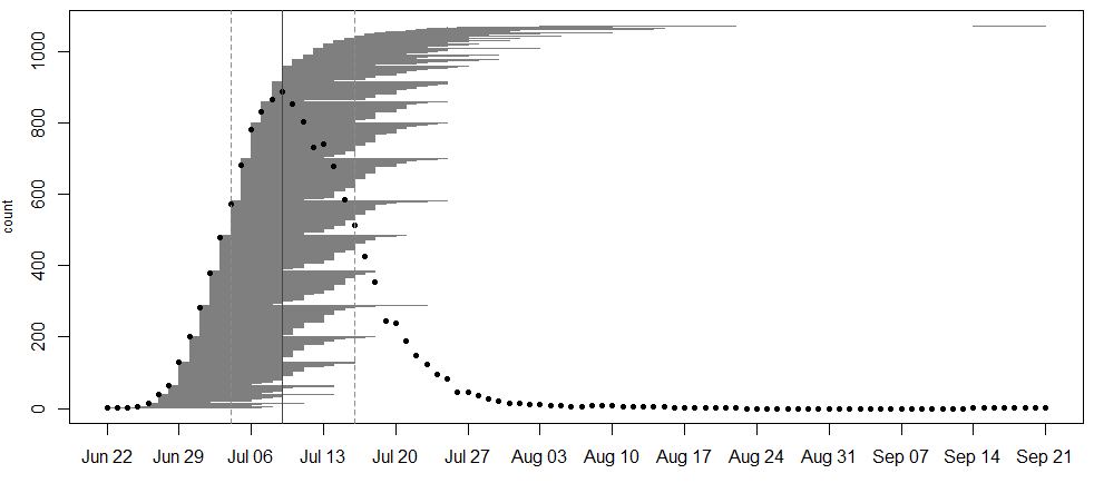
In 2020, we collected data on the timing of flowering for 855 flowering plants (1071 flowering heads) in 31 remnant populations. The plants ranged from having 1 to 8 flowering heads. The earliest bloomers initiated flowering on June 22nd . Plant 22195 at NWLF was the latest bloomer, only beginning to shed pollen on September 14th, nearly a month after the second-latest flowering plant had ceased producing pollen (August 18th). As is typical for the latest bloomer of a season, township mowers had mowed over this plant earlier in the season, which is perhaps why it took longer for it to sprout a new flowering stem. Peak flowering was on July 9th, when 886 heads were flowering.
A major part of the motivation behind this year’s effort in monitoring phenology was to collect baseline data on flowering rates and timing. Team Echinacea recently received funding to perform prescribed burns in these populations. Next summer, we will compare flowering patterns in populations before and after fires to understand how burns drive the effects of timing of flowering on mating patterns and fitness of individuals in natural populations.
Start year: 1996
Location: Roadsides, railroad rights of way, and nature preserves in and around Solem Township, MN
Overlaps with: phenology in experimental plots, demography in the remnants, gene flow in remnants, reproductive fitness in remnants
Data/materials collected: We identify each plant with a numbered tag affixed to the base and give each head a colored twist tie, so that each head has a unique tag/twist-tie combination, or “head ID”, under which we store all phenology data.We monitor the flowering status of all flowering plants in the remnants, visiting at least once every three days (usually every two days) until all heads were done flowering to obtain start and end dates of flowering. We managed the data in the R project ‘aiisummer2020′ and will add the records to the database of previous years’ remnant phenology records, which is located here: https://echinaceaproject.org/datasets/remnant-phen/. The dataset is ready to be updated, but I don’t believe it has been at the time of writing.
A flowering schedule for individuals from all remnants. Notice the gap between when second-to-last flower ceased pollen production and when the latest bloomer began on September 14th!
A flowering curve (created here using the R package mateable) summarizes the flowering phenology data that we collected in 2020, indicating the number of individuals flowering on a given day and the flowering period for all individuals over the course of the season.
We shot GPS points at all of the plants we monitored. Soon, we will align the locations of plants this year with previously recorded locations and given a unique identifier (‘AKA’). We will link this year’s phenology and survey records via the headID to AKA table.
You can find more information about phenology in the remnants and links to previous flog posts regarding this experiment at the background page for the experiment.
Products: A dataset of flowering phenology is ready to be posted on the website. It is currently located in Dropbox\remData\105_assessPhenology\phenology2020\phen2020_out and is available upon request. The headIds in this dataset have not yet been merged with the akas (long-term identifiers) in the demography dataset.
During the summer of 2019, Team Echinacea planted over 1400 E. angustifolia seedlings into 12 plots in a prairie restoration at West Central Area High School in Barrett, MN. We planted seedlings from three sources: (1) offspring from exPt1, (2) plants from my gene flow experiment, and (3) offspring from the Big Event. To test how different fire regimes affect fitness in Echinacea, folks from West Central Area plan to apply regular fall burn treatments to four plots, regular spring burn treatments to four other plots, and the remaining four plots will not be burned. I’m not sure if they were able to perform these burns as planned in Fall 2020 given COVID restrictions this spring and fall, but John Van Kempen would be the man to ask about that. I believe they were able to do the burns in the spring.
This summer, the team measured the 1-year old seedlings from my gene flow study in exPt10, as well as a few seedlings from the other plantings within the plot. The seedlings from my gene flow experiment are the offspring of open-pollinated Echinacea in 9 populations in the study area. I am assessing the paternity of these seedlings to understand contemporary pollen movement patterns within and among the remnants. In summer 2018, I mapped and collected leaf tissue from all Echinacea individuals within 800m of the study areas and harvested seedheads from a sample of these individuals (see Reproductive Fitness in Remnants). In spring 2019, I germinated and grew up a sample of the seeds that I harvested to obtain leaf tissue for genotyping.
Then, with the team’s help, I planted these seedlings in exPt10 in June 2019. I also collected seeds and leaf tissue in summer 2019 to repeat this process, but I did not germinate the achenes in the following spring because I was not able to assess seed set due to the broken x-ray machine at the CBG and then COVID-related restrictions. I hope to germinate those this spring and plant in summer 2021. I am working on extracting the DNA from the leaf tissue samples I have, which I will use to match up the genotypes of the offspring (i.e., the seeds) with their most likely father (i.e., the pollen source).
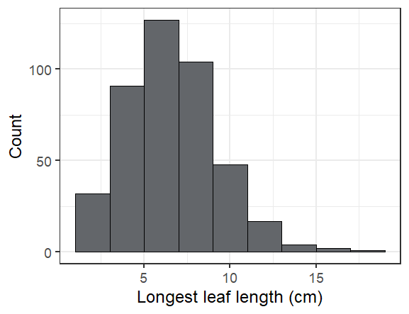
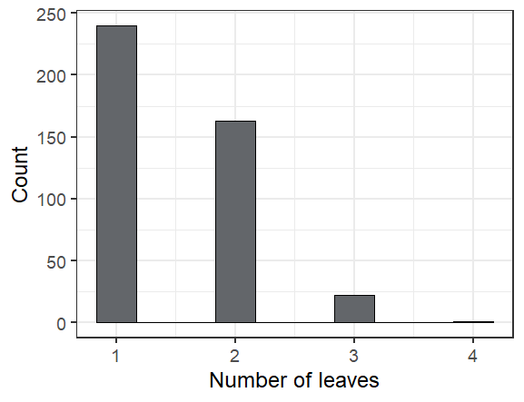
Here are some fun facts about the seedlings we found in exPt 10:
The longest leaf we saw was 19 cm! Most were much smaller (see below).
The leafiest plant we saw had 4 leaves (though one had been munched)
Overall we found 424 seedlings alive of the 598 that we searched for, or 71%. The ones we didn’t find are probably dead, but we’ll look for them again next year to make sure we didn’t just miss them.
I’m looking forward to seeing these friends again next year.
Allie gives a thumbs after successfully finding a baby Echinacea plant in p10!
Start year: 2018
Location: West Central Area High School’s Environmental Learning Center, Barrett, MN, Remnant prairies in Solem Township, Minnesota
This past Friday I planted the seeds from the inter-remnant crossing experiment I completed over the summer. The goal of this experiment is to understand how the distance between plants that live in little fragmented remnants and the difference in their timing of flowering influences the fitness of their offspring. The expectation is that if plants that are close together and/or flowering at the same time are closely related, their offspring might be more closely related (i.e., inbred) and have lower fitness than plants that are far apart and/or flowering more asynchronously. If this is true, then it would suggest that individuals in small, fragmented habitats would benefit from reaching more distant or dissimilar mates, such as by introducing seeds from faraway populations to remnants, creating corridors that promote pollinator movement, or managing habitat to increase heterogeneity in flowering time.
Plot location & layout:
The plot is located directly to the east of P1, spanning 12 m east to west and 30 m north to south, between positions 860 and 890. See Mia’s flog post from September for more information about how we prepared the plot by clipping the grass and treating the sumac with Garlon. Mia also used Darwin to shoot points within and along the edges of P1 so that I could generate coordinates for each position in my planting that aligned with P1’s crooked grid. This was a good exercise in geometry. I figured it out, but not before googling how to find the intersection of two lines. Oh well!
When I laid down the meter tapes based on the end points of the rows in this grid, it matched pretty well (the rows were supposed to be exactly 30 m long), but they were off a bit due to topography and the vegetation keeping the tape from laying perfectly flat. It was right on for row 58 and off by ~5cm in rows 62 and 65. We lined up meter sticks with the flags placed ever two meters and positioned achenes relative to according to the flag positions, rather than the tape. We placed 4 achenes per meter in positions 860-889.75.
Randomization:
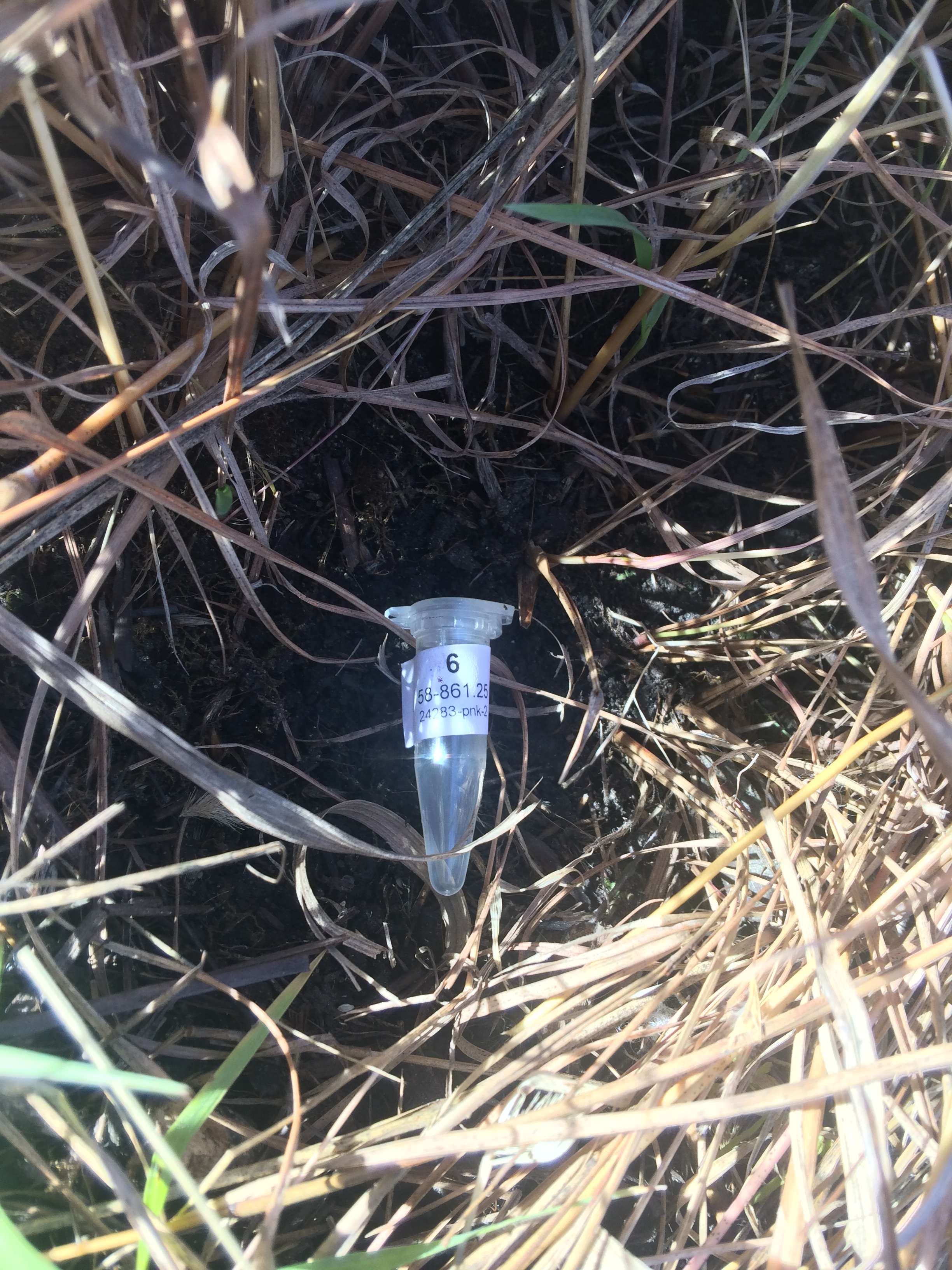
Based on the number of seeds I had, and the expectation that I might want to plant more for this experiment in the future, I randomly chose three rows (58, 62, and 65) to plant out of the twelve total rows that fit in the area that we prepared. I randomly assigned positions to all of the full achenes, based on their weight. Prior to planting, I placed each of these achenes into a 1.5mL microcentrifuge vial and labeled it with its planting position (1-360). I sorted the vials in order of planting position and placed them in vial trays that we brought into the field.
Planting:
It was a dry and unseasonably warm day. This is lucky because there was 10 inches of snow where the plot is located a week and a half earlier. I was able to convince Matthew and Gooseberry to come along to help. Matthew was extremely helpful, but Goose mostly ate deer poop all day and threw up on the way home. Very yucky! To set up for planting, I staked to the end points for the rows we were planting, set up a meter tape, and then staked to and placed pin flags at positions every two meters along the rows. I started by placing pin flags every meter, but this was time consuming and a pin flag every two meters gave us a sufficient reference point for each meter.
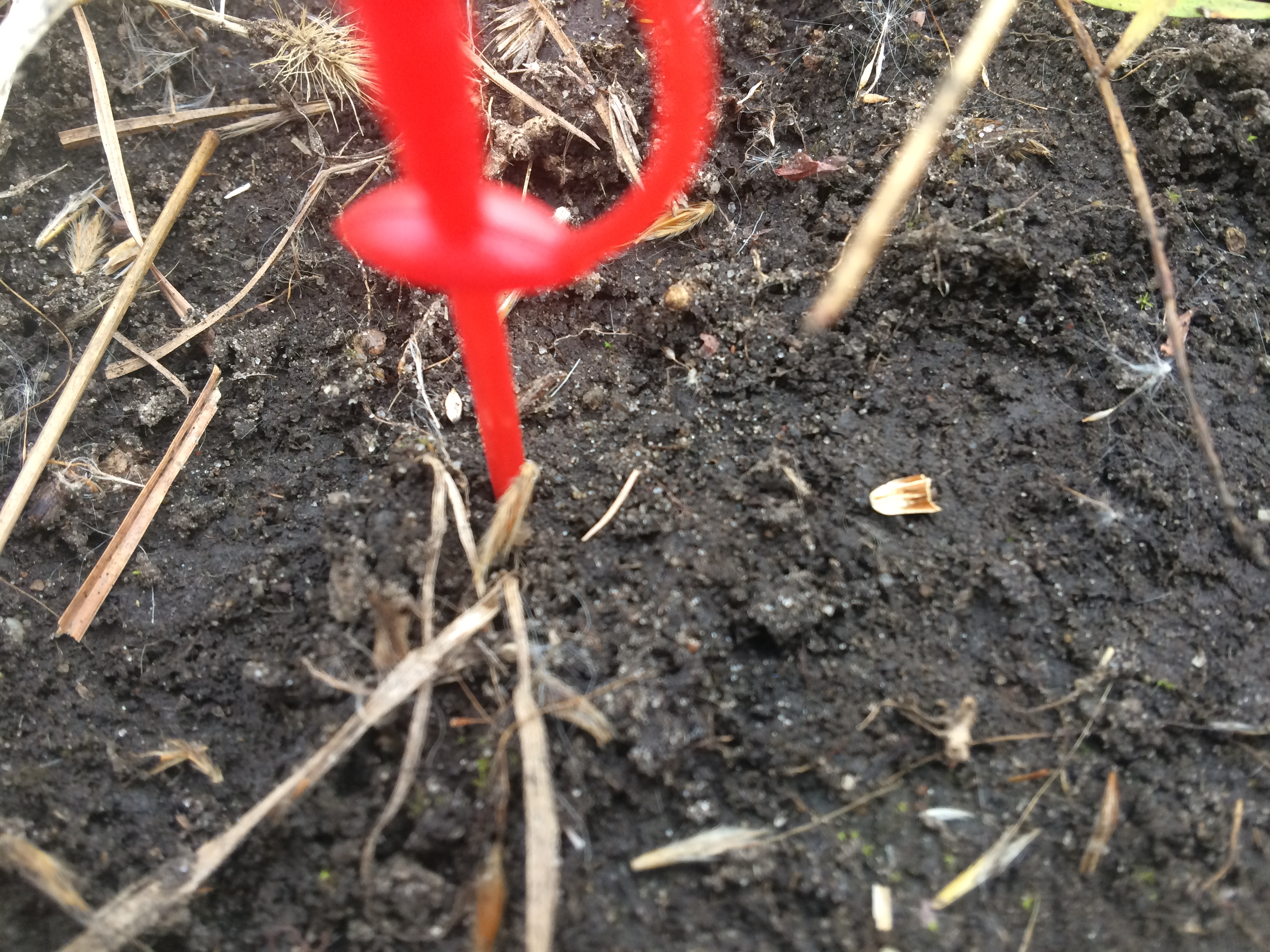
We liked breaking the actual planting into two steps, and working in a pair, because it meant that we had fewer items to fumble around with and it was easy to catch and fix each other’s mistakes, such as accidentally skipping positions. I do not believe we made any actual goofs, which is a first for me with planting! For the first step, one person cleared the duff, and the other placed the corresponding vial. For the second, one person placed the achene and collected the vial, while the other placed the toothpick and carried the clipboard, making any notes, e.g., if the achene was planted a few cm off the row to avoid placing it on a rock or in bunchgrass. The first step took about 10-12 minutes per 50 positions. The second took about 8-10 minutes per 50 positions. We set the achenes on top of the soil so that they had good contact with the soil, but weren’t buried. We finished around 4 PM and were grateful that we did not have to plant in the dark.
I hope the seeds have a good winter and I look forward to seeing them in the spring!
Team Echinacea continued the aphid addition and exclusion experiment started in 2011 by Katherine Muller. The original experiment included 100 plants selected from exPt01 which were each assigned to have aphids either added or excluded through multiple years. The intention is to assess the impact of the specialist herbivore Aphis echinaceae on Echinacea fitness.
The 2020 aphid team was Anna Allen and Allie Radin. They located 25 living exclusion plants and 16 living addition plants. The experiment was conducted from July 6th to August 19th, with the final visit consisting only of observation. Aphids were moved only during four visits from late July to mid-August due to late arrival and low numbers of aphids. Only one or two aphids were applied to each plant during each visit. They recorded the number of aphids present in classes of 0, 1, 2-10, 11-80, and >80. They also recorded the number of aphids added.
Aphids on an Echinacea leaf
Start year: 2011 Location: Experimental Plot 1 Overlaps with: Phenology and fitness in P1 Data collected: Scanned datasheets are located at ~Dropbox\teamEchinacea2020\allisonRadin\aphidAddEx2020.
Products:
Andy Hoyt’s poster presented at the Fall 2018 Research Symposium at Carleton College
2016 paper by Katherine Muller and Stuart on aphids and foliar herbivory damage on Echinacea
2015 paper by Ruth Shaw and Stuart on fitness and demographic consequences of aphid loads
You can read more about the aphid addition and exclusion experiment, as well as links to prior flog entries mentioning the experiment, on the background page for this experiment.
I wanted to make a post detailing my experiment this summer with hybrid Echinacea plants at Hegg Lake. As a student, it was my goal to design, execute, and analyze an experiment with Team Echinacea this summer. Because I’m interested in genetics, I wanted to create something that would connect inheritance with population control among Echinacea. With the help of some seasoned Team Echinacea members (Riley T and Mia S), I was able to construct an experiment that would study the reproduction potential of hybrid Echinacea, crossed between E. angustifolia and E. pallida.
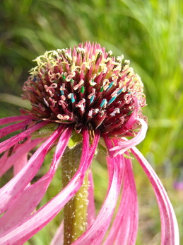
In the history of experimental plot 7, two Echinacea plants have flowered. Most recently, a hybrid Echinacea flowered this spring. This allowed us to cross the hybrid’s pollen with a variety of E. angustifolia and E. pallida in the Hegg Lake area. In order to assess reproduction potential, styles were painted, pollinated, and later observed to look for shriveling. Although styles may shrivel for a variety of reasons, shriveling usually indicates reproduction. In the winter, we will assess the seed-set of these individuals to determine reproductive fitness.
When new species from non-prairie remnants are introduced to new areas, the risk of hybridization among plants of the same genus arises. E. pallida, which has shown to out-compete E. angustifolia in our experimental plots, therefore has the ability to pass on its genes through hybrids. If hybrids are able to reproduce, and continue to pass on E. pallida genes, the risks of genetic swamping increase. Therefore, over time, hybridization could eventually exterminate E. angustifolia from its native prairie.
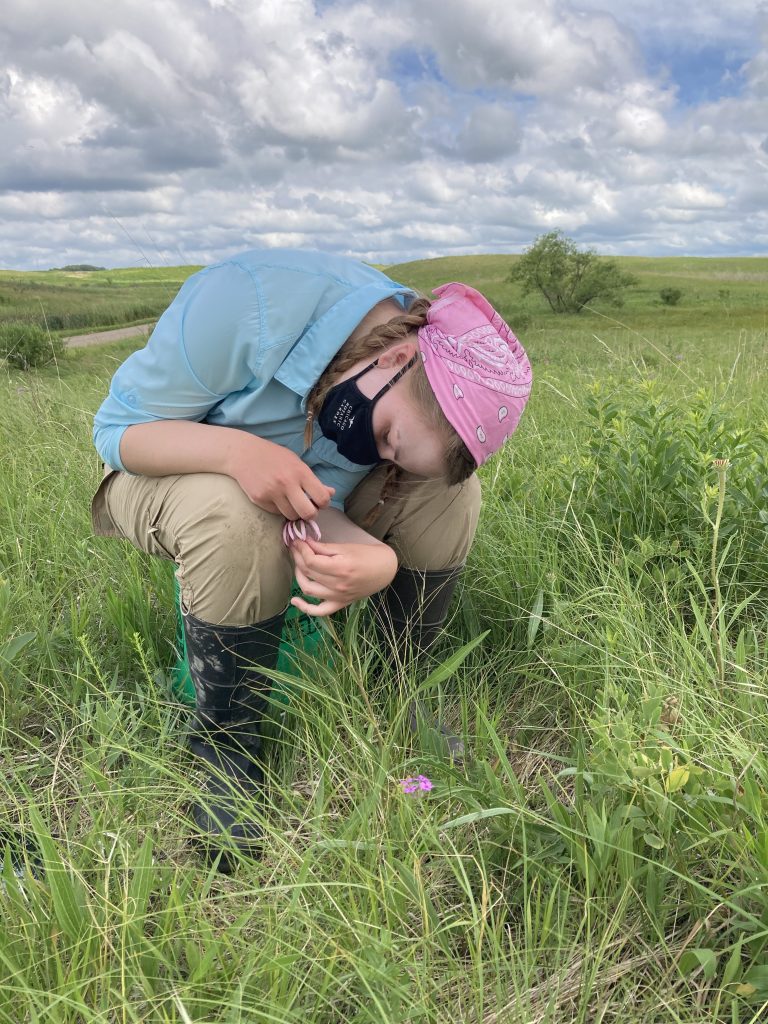
A picture of me painting bracts for our hybrid crosses. Photo credit to Mia S!
In order to assess reproduction, we hand-crossed a variety of sample pollen with E. angustifolia, E. pallida, and hybrid Echinacea. In this experiment, a shriveled style is a sign of successful reproduction. Because Echinacea plants are not self-compatible, the reasons for a style not to shrivel could vary. Reasons could be that the hybrid was not compatible with this type of Echinacea, or because the specific Echinacea plants were incompatible due to inheritance patterns.
An example of hand-crosses from Shona Sanford-Long, 2012
Our sample size was also effected because only one hybrid Echinacea flowered this summer. In the end, we cross-pollinated our hybrid plant with three E. angustifolia plants, and three E. pallida plants. If more hybrids flower in the future, we will be able to expand our sample size and cross variety. For this reason, we hope to continue this experiment in the following summers if hybrids continue to flower.
Overall, we saw that hybrids were more compatible with E. angustifolia rather than E. pallida. While hybrid reproduction passes on E. pallida genes, a greater chance of reproduction with E. angustifolia keeps native genes (and hopefully, native traits) in the prairie gene pool.
In the future, I will share more updates as we continue to analyze and reassess the data.
Thanks for joining me on this exciting, new experiment!
Supplemental pollen — pollen that an Echinacea head might not otherwise receive—could increase a plant’s fitness. But does this extra pollination lead to a tradeoff in survival or flowering consistency? Since 2012, we have been manipulating the amount of pollen Echinacea plants receive – either no pollen, or lots of pollen – and recording how this affects their fitness and survival. In 2012 and 2013 we identified flowering E. angustifolia plants in experimental plot 1 and randomly assigned one of two treatments to each: pollen addition or pollen exclusion. The team bagged the heads of all plants and hand-pollinated the addition treatment, and did not manipulate the exclusion plants further. Plants receive the same treatment across years.
In summer 2018, 14 of the 26 plants alive in the pollen addition and exclusion experiment flowered, producing a total of 25 heads. This year none of those plants flowered. Of the original 38 plants in this experiment, 12 of the exclusion plants and 14 of the pollen addition plants are still alive. No plants died between 2018 and 2019. This year’s data were unique among the eight years of data collected, because not a single plant in the experiment produced even a single head. The dramatic decrease in flowering rates this year may help or hinder us in analyzing this data set and providing answers to this eight-year question.
Tris did not find significant demographic differences between plants which received pollen exclusion, addition or open pollination treatments.
Start year: 2012
Location: exPt1
Physical specimens: We harvested no specimens this year
Data collected: Plants survival and measurements were recorded as part of our annual surveys in P1 and can be found with the rest of the P1 data in the R package EchinaceaLab.
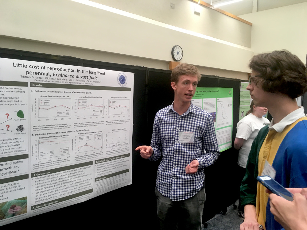
Michael presented a poster on the polLim experiment at MEEC
2019, which you can find here
Tris also presented a poster on polLim at MEEC 2019, which you can find here
You can find more information about the pollen addition and
exclusion experiment and links to previous flog posts regarding this
experiment at the background page for the experiment.
Team Echinacea established quantitative genetics experiments to determine the additive genetic variance of fitness in Echinacea, with the idea that we can estimate evolutionary potential of study populations. Quantitative genetics experiments 2 and 3 (qGen2 and qGen3) represent the third generation of Echinacea in our common garden experiments. The grandparents of qGen2 and qGen3 are the 1996 and 1997 gardens. Plants from these experiments were crossed to generate qGen1 (a.k.a. Big Batch), and plants in qGen1 were crossed to produce seed for qGen2 and qGen3, which now inhabit exPt8.
We visit exPt8 every year to assess fitness of Echinacea in the plot. Originally, 12,813 seeds were sown in the common garden. Seeds from the same maternal and paternal plant were sown in meter-long segments between nails. A total of 3253 seedlings were originally found, but only 669 plants were found alive in 2019.
Jay, John, and Avery assess fitness of young Echinacea in exPt8. They’re so tiny (the Echinacea, that is… Jay, John, and Avery are regular sized).
In an exciting turn of events, we found a flowering plant in qGen2 this year! This was the first flowering plant found in exPt8. Fortunately for our one flowering plant, it had four flowering friends to cross with from the Transplant Plot. We took phenology data on the qGen2 head, measured it, and harvested it.
The presence of a flowering plant influenced Riley Thoen to make a new measuring form for exPt8 in 2020. In the past, the exPt8 measuring form was very different from other measuring forms. Through 2019, we measured all leaves of basal plants in exPt8; we only measure the longest basal leaf in other plots. Riley designed the 2020 exPt8 measuring form to mirror the measuring forms from other common gardens. In the future, the exPt8 measure form will have a head subform and team members will only have to measure the longest basal leaf of each plant found.
Start Year: 1996 and 1997 (Grand-dams), 2003 (qGen1 – dams), 2013 and 2015 (qGen2 and qGen3, respectively)
Data/material collected: phenology data on the flowering plant and transplant plot plants (available in the exPt1 phenology data frames in the cgData repo), measure data (cgData repo), and harvested heads (data available in hh.2019 in the echinaceaLab package; heads in ACE protocol at CBG).
The inbreeding 2 experiment was planted in exPt1 in 2006 to determine how genetic drift is differentially affecting average fitness of remnant populations. In 2005, team members crossed common garden plants from seven remnant populations. There are three cross types: inbred (crossed to a half-sib; I), within population (randomly chosen; W), and between population (B). Each year, team members assess flowering phenology and fitness of Echinacea in the inb2 common garden.
In 2019, the team searched for Echinacea at 508 positions of the original 1443 positions planted in inb2. In total, we found 351 living plants. Four plants flowered in 2019 but only three produced achenes. Since 2006, 163 Echinacea in inb2 have flowered; they have produced a total of 336 flowering heads.
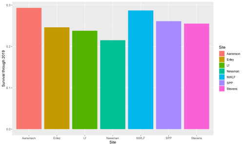
This winter, Riley Thoen is working on analyzing data and drafting a manuscript for inb2. In these endeavors, he found a small discrepancy in inb2 data: not all plants that were planted in the inb2 plot have a complete pedigree. Therefore, only a subset of the total can be used for analysis. A total of 1136 plants with a complete pedigree were planted in inb2, and of those, 277 were found alive in 2019. All four plants that flowered in 2019 have known pedigrees. A total of 138 plants of known pedigree have flowered and they have produced 284 total heads since the plot was planted in 2006. Surprisingly, within-remnant crosses have the lowest survival of all cross types, at 20%. Inbred crosses have 24% survival and between-remnant crosses have 30% survival. Riley is starting to push data analysis forwards and will certainly post updates on the flog when more discoveries are made!
Data/material collected: flowering phenology on the flowering plants (available in the exPt1 phenology data frames in the cgData repo), measure data (cgData repo), and harvested heads (data available in hh.2019 in the echinaceaLab package; heads in ACE protocol at CBG).
Products:
Shaw, R. G., S. Wagenius and C. J. Geyer. 2015. The susceptibility of Echinacea angustifolia to a specialist aphid: eco-evolutionary perspective on genotypic variation and demographic consequences. Journal of Ecology 103: 809-818. PDF
Kittelson, P., S. Wagenius, R. Nielsen, S. Qazi, M. Howe, G. Kiefer, and R. G. Shaw. 2015. Leaf functional traits, herbivory, and genetic diversity in Echinacea: Implications for fragmented populations. Ecology 96: 1877–1886. PDF