In summers 2018 and 2019, I mapped and collected leaf tissue from all individuals in the study areas and harvested seedheads from a subset of Echinacea individuals at populations in the NW corner of the study area (populations: ALF, EELR, KJ, NWLF, GC, SGC, NGC, KJ, NNWLF) to map pollen movement (see Reproductive Fitness in Remnants). To analyze patterns of gene flow, I will assess how individuals’ location and timing of flowering influence their reproductive success and distance of pollen movement. I am currently wrapping up genotyping the DNA from the leaf tissue samples and a subset of the seeds I collected. This summer, the team measured the 3-year-old seedlings from the gene flow study that are planted in exPt10. I did not do additional field work for this project this year.
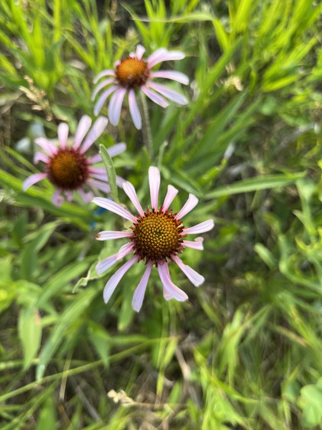
A flowering Echinacea angustifolia
Start year: 2018
Location: Roadsides, railroad rights of way, and nature preserves in and around Solem Township, MN
Data collected: exPt10 measure data is in the cgdata repo.
Products: I presented a poster based on the locations and flowering phenology of individuals from summer 2018 at the International Pollinator Conference in Davis, CA this summer. The poster is linked here: https://echinaceaproject.org/international-pollinator-conference/.
In summer 2022, I continued the interremnant crosses experiment to understand how the distance between plants in space and their timing of flowering influences the fitness of their offspring. This experiment builds on my study of gene flow and pollen movement in the remnants, asking the question of how pollen movement patterns affect offspring establishment and fitness. If plants that are located close together or flower at the same time are closely related, their offspring might be more closely related and inbred, and have lower fitness than plants that are far apart and/or flower more asynchronously. In other words, if distance in space or time is correlated with relatedness, we’d expect mating between more distant or asynchronous individuals to result in more fit offspring.
To test this hypothesis, I performed crosses between plants across a range of spatial isolation (within the same population, in adjacent populations, and in far-apart populations) in 2020. With the team’s help, I also kept track of the individuals’ flowering time to assess whether reproductive synchrony is associated with reduced offspring fitness, suggesting that individuals that flower at the same time are more closely related.
In 2021, I repeated the same hand crossing methods to assess the fitness consequences of outcrossing on 44 focal plants. However, instead of planting the offspring from these crosses as seeds, I germinated them in the growth chamber and transferred sprouts to a plug tray.
In spring 2022, with help from the team, I planted the seedlings as plugs into ExPt1. I measured the seedlings throughout the summer.
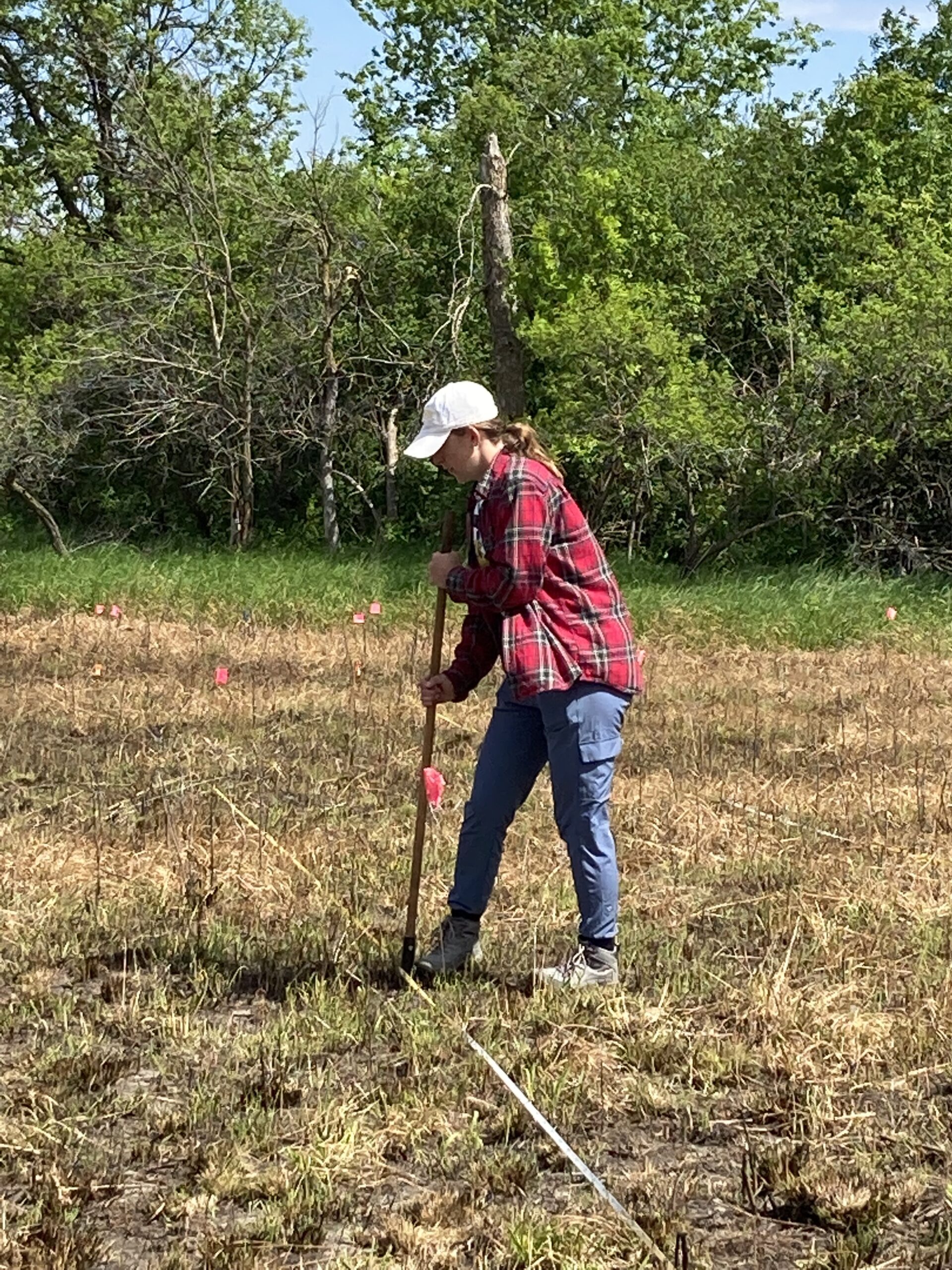
Lindsey digs a hole for an Echinacea plugA baby Echinacea!Amy plants Echinacea in ExPt1 after the burn
To learn more about Amy’s project, check out this video created by 2021 RET participant Alex Wicker.
Start year: 2020
Location: On27, SGC, GC, NGC, EELR, KJ, NNWLF, NWLF, LF
Data collected: Style shriveling and seed set and weight from crosses, start and end date of flowering, coordinates of all individuals in the populations listed above. Leaf count and height of seedlings at three points during the summer (two weeks after planting, mid-summer, and late summer).
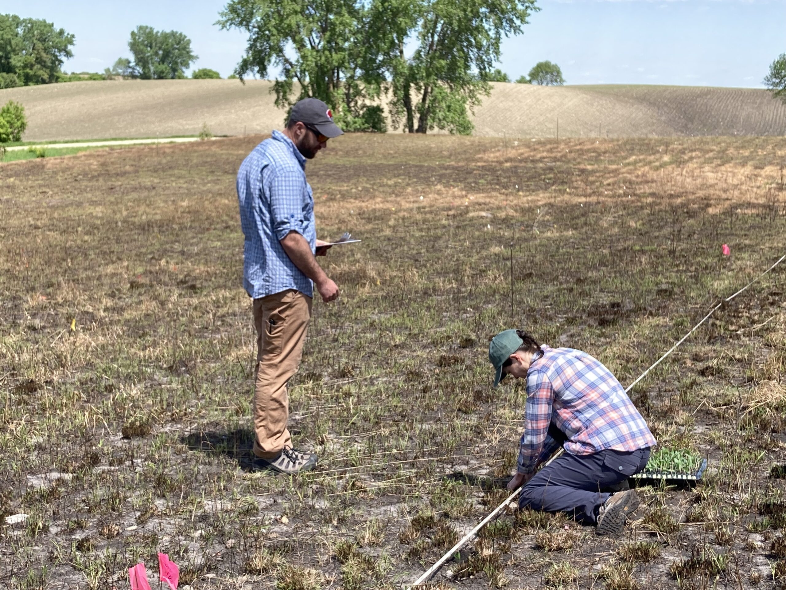
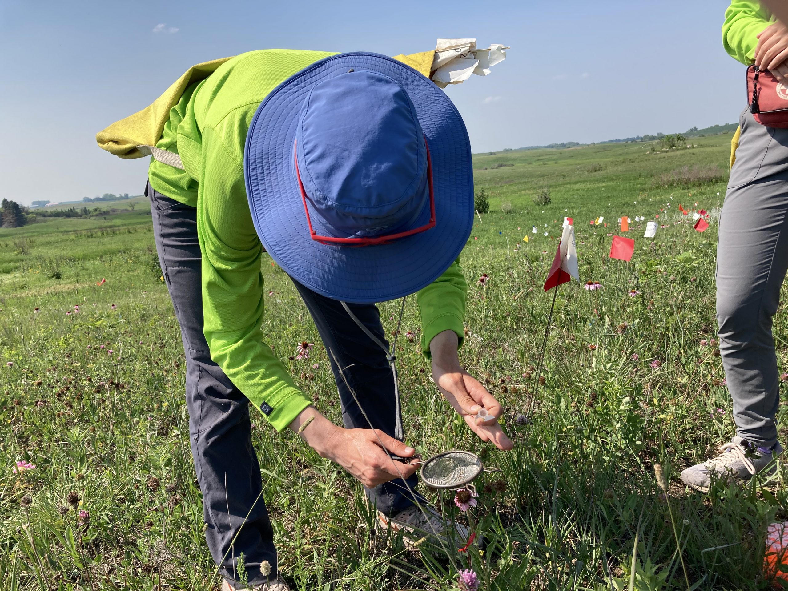
In summer 2021, we began a project to look at the effect of dust on reproduction of Echinacea. We randomly assigned treatments of ‘dust’ or ‘no dust’ to 41 heads in ExPt2 that were on first or second-day of flowering at the onset of our treatments. For ‘dust’ plants, we applied ~1g dust with a sifter to the top of each head at least once every three days until the heads were no longer flowering. Team Dust consisted of Emma, Alex, Kennedy, Mia, and I. We harvested the treatment heads at the end of the season. Unfortunately, we were only able to harvest 18 seedheads due to rodent herbivory. We will evaluate their seed set in Winter 2022.
Amy sifts dust on to an Echinacea head
Start year: 2021
Location: ExPt2
Overlaps with: None
Data collected: We collected style persistence data from treatment seedheads. Data has been double-entered and verified and is located in Dropbox/teamEchinacea2021/teamDust/p2DustTreatments_de.csv
Samples or specimens collected: We collected 18 seedheads, which are currently in the R. Shaw Lab in the Ecology building at UMN.
Products: None yet!
You can read more about the dust experiment in flog entries from summer 2021.
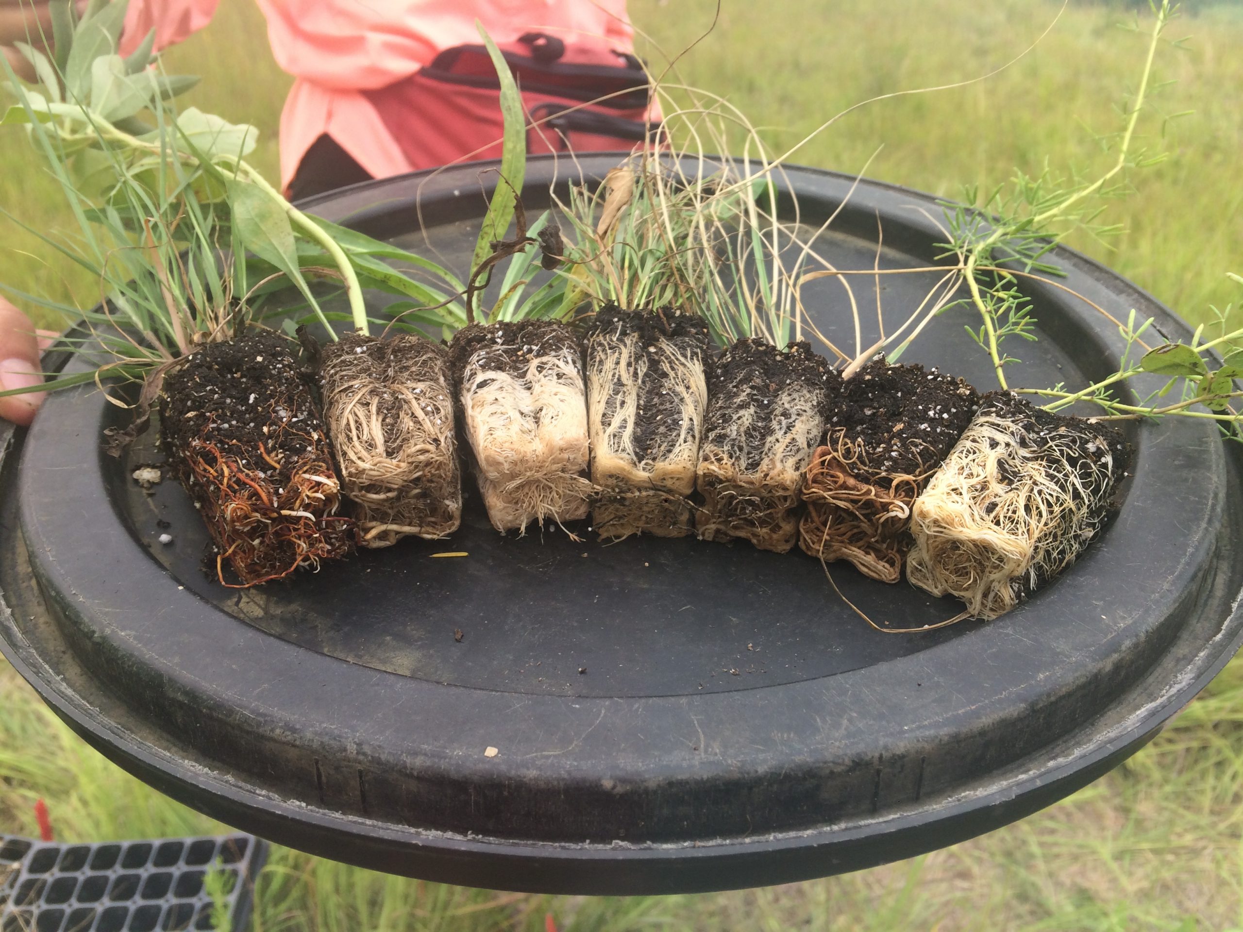
During the summer of 2019, Team Echinacea planted over 1400 E. angustifolia seedlings into 12 plots in a prairie restoration at West Central Area High School in Barrett, MN. We planted seedlings from three sources: (1) offspring from exPt1, (2) plants from my gene flow experiment, and (3) offspring from the Big Event. In summer 2021, Drake also planted plugs of other species (pictured below).
This summer, the team measured the 2-year old seedlings from my gene flow study in exPt10, as well as a few seedlings from the other plantings within the plot. The seedlings from my gene flow experiment are the offspring of open-pollinated Echinacea in 9 populations in the study area. I am assessing the paternity of these seedlings to understand contemporary pollen movement patterns within and among the remnants. In summer 2018, I mapped and collected leaf tissue from all Echinacea individuals within 800m of the study areas and harvested seedheads from a sample of these individuals (see Reproductive Fitness in Remnants). In spring 2019, I germinated and grew up a sample of the seeds that I harvested to obtain leaf tissue for genotyping.
Then, with the team’s help, I planted these seedlings in exPt10 in June 2019. I also collected seeds and leaf tissue in summer 2019 to repeat this process, but I did not germinate the achenes in the following spring because I was not able to assess seed set due to the broken x-ray machine at the CBG and then COVID-related restrictions. I hope to germinate those this spring and plant in summer 2022. I am working on extracting the DNA from the leaf tissue samples I have, which I will use to match up the genotypes of the offspring (i.e., the seeds) with their most likely father (i.e., the pollen source).
A sampler platter of seedlings, planted as part of Drake’s study of how prairie communities respond to parasitic plants.
Start year: 2018
Location: West Central Area High School’s Environmental Learning Center, Barrett, MN, Remnant prairies in Solem Township, Minnesota
Another busy day for Team Echinacea! I started field work late this morning due to giving a talk at the virtual Evolution conference. Everything was pre-recorded, so it was great to enjoy listening to all the other talks in my session and learn about some new ideas related to gene flow. The title of my talk was “Outcrossing distance in space and time affects fitness in a long-lived perennial” — I’m planning to post the video on the Team Echinacea YouTube channel sometime soon so you can watch it anytime. While I was watching talks, the team was busy at work, doing phenology, shooting points, and nearly finishing flowering demo at all of the sites.
At lunch, we discussed team norms. Stuart floated the idea of turning the team norms into a blood pact sort of thing, but there was not much enthusiasm for the idea. It’s okay because one of our norms is that we want our work environment to be a “soft space” where everyone feels welcome to share their ideas, even if others don’t share the same opinion!
After lunch was the inaugural meeting of Team Dust. This is an exciting new initiative to investigate the effects of road dust on Echinacea. How much dust from gravel roads winds up landing on the plants on roadsides? Does this dust affect pollination or seed set? We intend to find out!
Here is a picture of several color-coordinated members of Team Dust.
Finally, we had our second official social gathering of the season. We ate bean burgers, air-fried fries, and (my personal favorite) Jean’s famous brownies! Delicious. We also drank and discussed several flavors of iced tea. Some of the words used to describe one of the teas included “turpentine”, “pine-sol”, “earthy”, and “savory”. Can you guess which one?
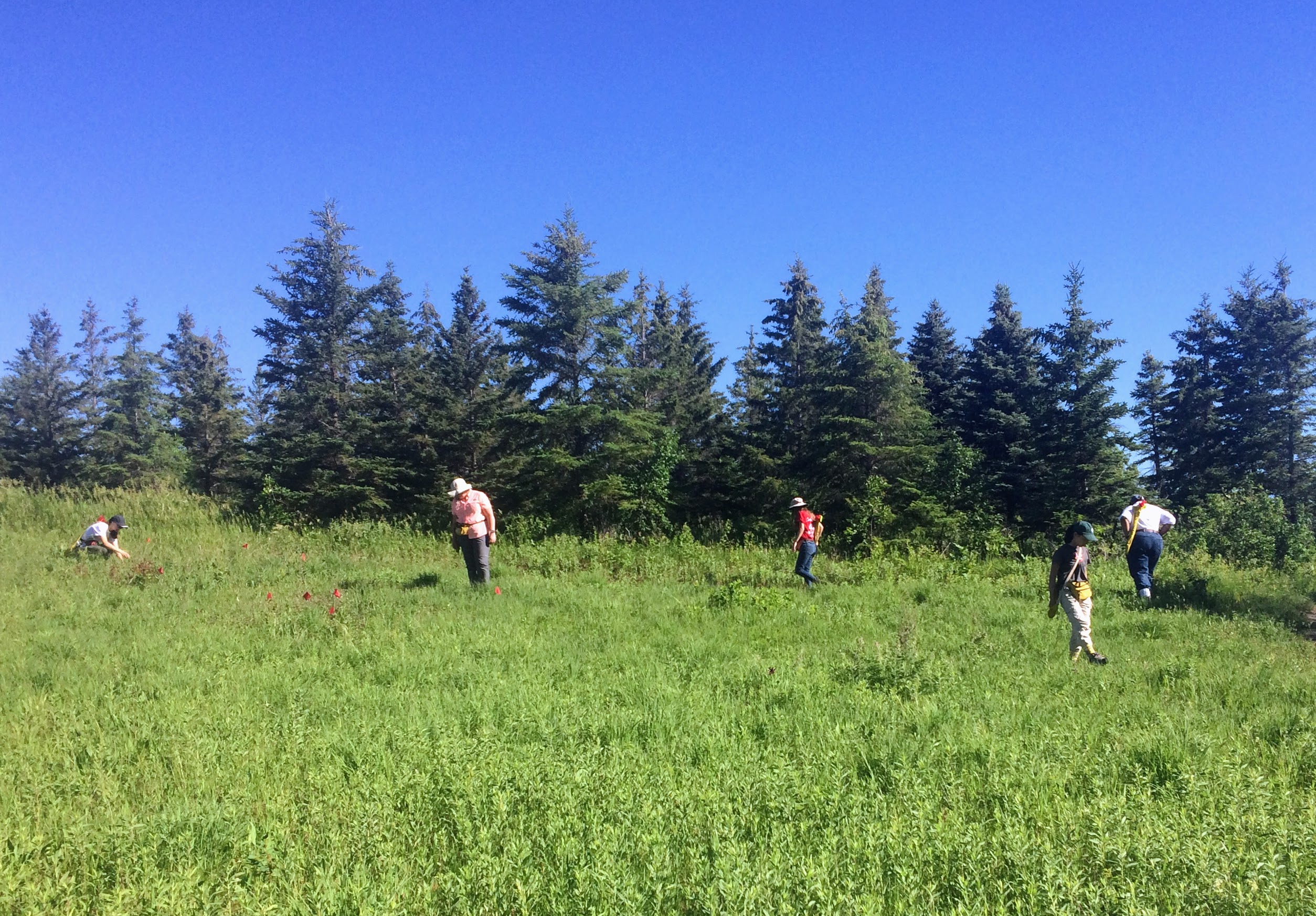
What’s up, flogland! Today was day two of the field season for Team Echinacea. In the morning, Jared, Allie, Maris, Emma, Alex, and I went to KJ’s to learn how to search for flowering Echinacea and how to make demo records. We found and made records for 43(!) flowering plants at KJ’s and then went to search for more at East Elk Lake Road. At lunch, Ruth presented a talk about the entanglement of environment and genetics in the expression of traits and Jared presented some of the background for the experiment looking at the effects of fire on reproduction in the remnants. After lunch, while the rest of the team either learned how to use the GPS or flagged P1, I went out to some of the sites in the northwest corner of the study area (where I’ll do my crossing experiment this summer) to search for and flag more flowering plants. I’m sure there are plants that I missed, but I hope this helps us get a good start! Here are the totals for flowering plants I found at each site: South of Golf Course – 15, Golf Course – 9, North of Golf Course – 2, North of Northwest of Landfill – 9, and Northwest of Landfill – 14.
This summer I started a new experiment to understand how the distance between plants in space and in their timing of flowering influences the fitness of their offspring. This experiment builds on my study of gene flow and pollen movement in the remnants, asking the question of how pollen movement patterns affect offspring establishment and fitness. If plants that are located close together or flower at the same time are closely related, their offspring might be more closely related and inbred, and have lower fitness than plants that are far apart and/or flower more asynchronously. In other words, if distance in space or time is correlated with relatedness, we’d expect mating between more distant or asynchronous individuals to result in more fit offspring.
To test this hypothesis, I performed crosses between plants across a range of spatial isolation (within the same population, in adjacent populations, and in far-apart populations). With the team’s help, I also kept track of the individuals flowering time so that I can assess whether reproductive synchrony is associated with reduced offspring fitness, suggesting that individuals that flower at the same time are more closely related.
I ended up using 42 focal plants (two of which were mowed before I could harvest them) and a total of 167 sires. I planted 359 offspring from these crosses in November. Next spring and summer, I will measure the seedlings to collect data on emergence and growth. Seed set was lower than I wanted it to be (only ~20%, when I would have expected 60-70% based on compatibility rates in the remnants), so I will also likely perform more crosses in summer 2021 to shore up my sample size.
Crossing at scenic On 27
Start year: 2020
Location: On27, SGC, GC, NGC, EELR, KJ, NNWLF, NWLF, LF
Data/Materials collected: 40 seedheads, style shriveling and seed set and weight from crosses, start and end date of flowering, coordinates of all individuals in the populations listed above
Products: I planted the seeds from the crosses in a plot adjacent to P1 in November, as detailed in this flog post.
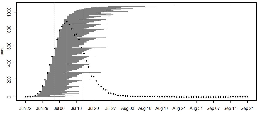
In 2020, we collected data on the timing of flowering for 855 flowering plants (1071 flowering heads) in 31 remnant populations. The plants ranged from having 1 to 8 flowering heads. The earliest bloomers initiated flowering on June 22nd . Plant 22195 at NWLF was the latest bloomer, only beginning to shed pollen on September 14th, nearly a month after the second-latest flowering plant had ceased producing pollen (August 18th). As is typical for the latest bloomer of a season, township mowers had mowed over this plant earlier in the season, which is perhaps why it took longer for it to sprout a new flowering stem. Peak flowering was on July 9th, when 886 heads were flowering.
A major part of the motivation behind this year’s effort in monitoring phenology was to collect baseline data on flowering rates and timing. Team Echinacea recently received funding to perform prescribed burns in these populations. Next summer, we will compare flowering patterns in populations before and after fires to understand how burns drive the effects of timing of flowering on mating patterns and fitness of individuals in natural populations.
Start year: 1996
Location: Roadsides, railroad rights of way, and nature preserves in and around Solem Township, MN
Overlaps with: phenology in experimental plots, demography in the remnants, gene flow in remnants, reproductive fitness in remnants
Data/materials collected: We identify each plant with a numbered tag affixed to the base and give each head a colored twist tie, so that each head has a unique tag/twist-tie combination, or “head ID”, under which we store all phenology data.We monitor the flowering status of all flowering plants in the remnants, visiting at least once every three days (usually every two days) until all heads were done flowering to obtain start and end dates of flowering. We managed the data in the R project ‘aiisummer2020′ and will add the records to the database of previous years’ remnant phenology records, which is located here: https://echinaceaproject.org/datasets/remnant-phen/. The dataset is ready to be updated, but I don’t believe it has been at the time of writing.
A flowering schedule for individuals from all remnants. Notice the gap between when second-to-last flower ceased pollen production and when the latest bloomer began on September 14th!
A flowering curve (created here using the R package mateable) summarizes the flowering phenology data that we collected in 2020, indicating the number of individuals flowering on a given day and the flowering period for all individuals over the course of the season.
We shot GPS points at all of the plants we monitored. Soon, we will align the locations of plants this year with previously recorded locations and given a unique identifier (‘AKA’). We will link this year’s phenology and survey records via the headID to AKA table.
You can find more information about phenology in the remnants and links to previous flog posts regarding this experiment at the background page for the experiment.
Products: A dataset of flowering phenology is ready to be posted on the website. It is currently located in Dropbox\remData\105_assessPhenology\phenology2020\phen2020_out and is available upon request. The headIds in this dataset have not yet been merged with the akas (long-term identifiers) in the demography dataset.
During the summer of 2019, Team Echinacea planted over 1400 E. angustifolia seedlings into 12 plots in a prairie restoration at West Central Area High School in Barrett, MN. We planted seedlings from three sources: (1) offspring from exPt1, (2) plants from my gene flow experiment, and (3) offspring from the Big Event. To test how different fire regimes affect fitness in Echinacea, folks from West Central Area plan to apply regular fall burn treatments to four plots, regular spring burn treatments to four other plots, and the remaining four plots will not be burned. I’m not sure if they were able to perform these burns as planned in Fall 2020 given COVID restrictions this spring and fall, but John Van Kempen would be the man to ask about that. I believe they were able to do the burns in the spring.
This summer, the team measured the 1-year old seedlings from my gene flow study in exPt10, as well as a few seedlings from the other plantings within the plot. The seedlings from my gene flow experiment are the offspring of open-pollinated Echinacea in 9 populations in the study area. I am assessing the paternity of these seedlings to understand contemporary pollen movement patterns within and among the remnants. In summer 2018, I mapped and collected leaf tissue from all Echinacea individuals within 800m of the study areas and harvested seedheads from a sample of these individuals (see Reproductive Fitness in Remnants). In spring 2019, I germinated and grew up a sample of the seeds that I harvested to obtain leaf tissue for genotyping.
Then, with the team’s help, I planted these seedlings in exPt10 in June 2019. I also collected seeds and leaf tissue in summer 2019 to repeat this process, but I did not germinate the achenes in the following spring because I was not able to assess seed set due to the broken x-ray machine at the CBG and then COVID-related restrictions. I hope to germinate those this spring and plant in summer 2021. I am working on extracting the DNA from the leaf tissue samples I have, which I will use to match up the genotypes of the offspring (i.e., the seeds) with their most likely father (i.e., the pollen source).
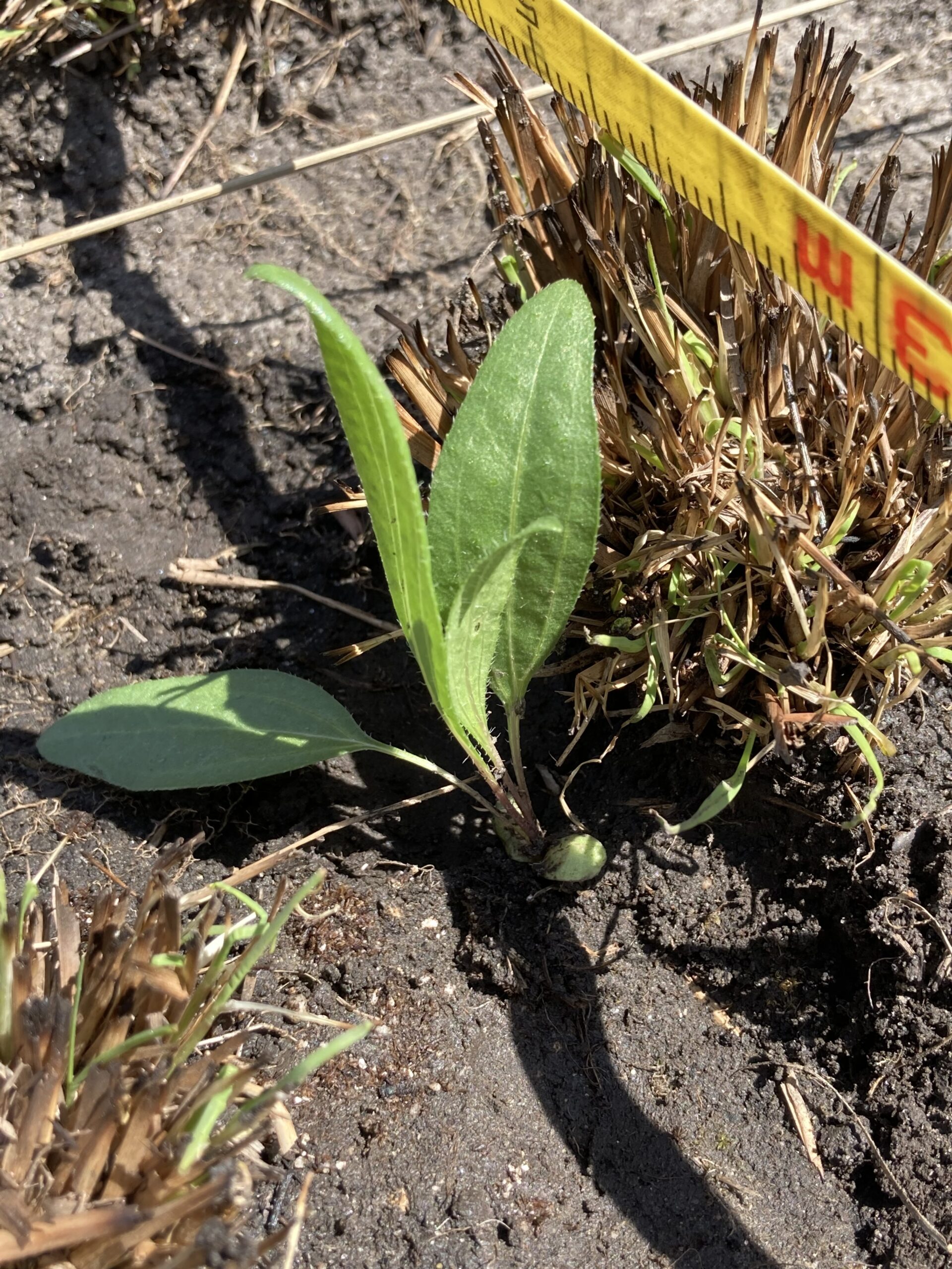
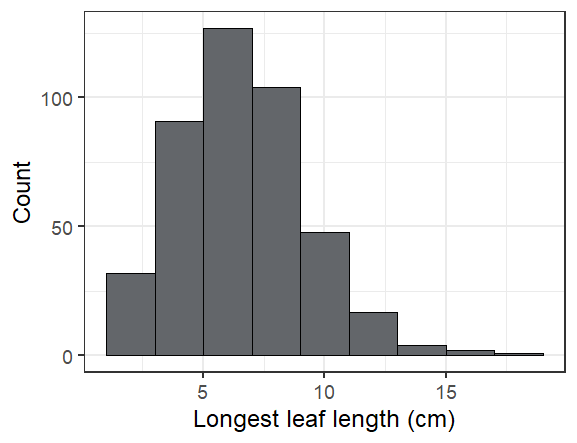
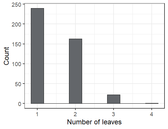
Here are some fun facts about the seedlings we found in exPt 10:
The longest leaf we saw was 19 cm! Most were much smaller (see below).
The leafiest plant we saw had 4 leaves (though one had been munched)
Overall we found 424 seedlings alive of the 598 that we searched for, or 71%. The ones we didn’t find are probably dead, but we’ll look for them again next year to make sure we didn’t just miss them.
I’m looking forward to seeing these friends again next year.
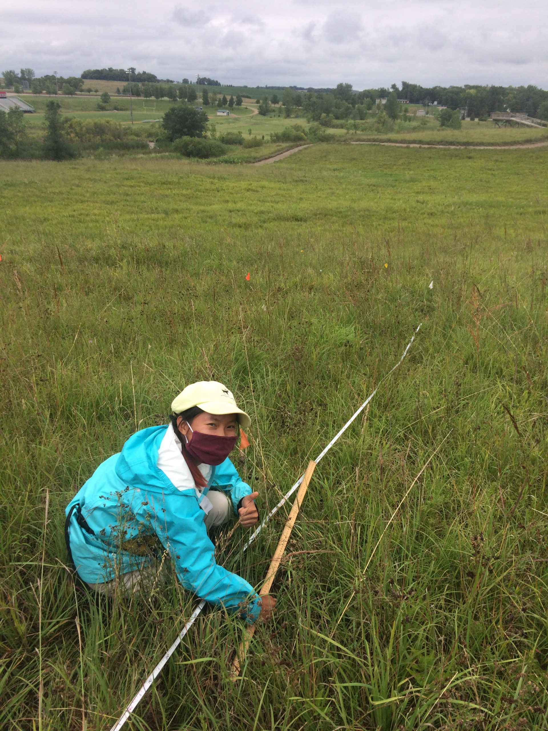
Allie gives a thumbs after successfully finding a baby Echinacea plant in p10!
Start year: 2018
Location: West Central Area High School’s Environmental Learning Center, Barrett, MN, Remnant prairies in Solem Township, Minnesota
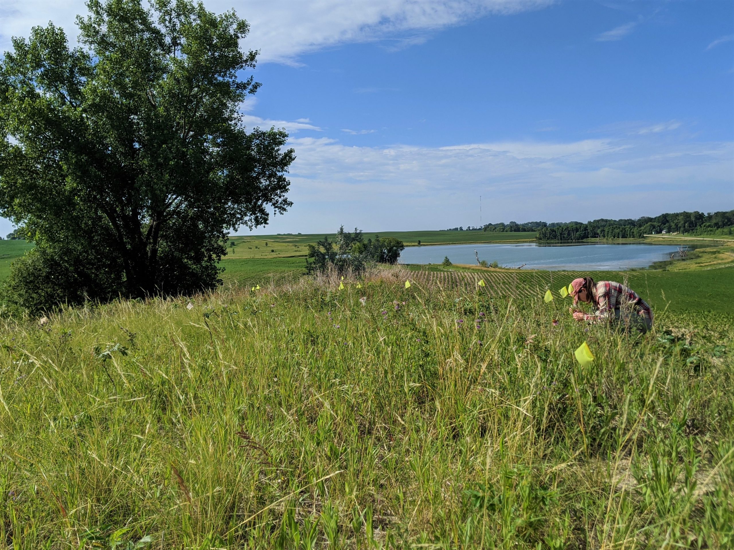
This past Friday I planted the seeds from the inter-remnant crossing experiment I completed over the summer. The goal of this experiment is to understand how the distance between plants that live in little fragmented remnants and the difference in their timing of flowering influences the fitness of their offspring. The expectation is that if plants that are close together and/or flowering at the same time are closely related, their offspring might be more closely related (i.e., inbred) and have lower fitness than plants that are far apart and/or flowering more asynchronously. If this is true, then it would suggest that individuals in small, fragmented habitats would benefit from reaching more distant or dissimilar mates, such as by introducing seeds from faraway populations to remnants, creating corridors that promote pollinator movement, or managing habitat to increase heterogeneity in flowering time.
Plot location & layout:
The plot is located directly to the east of P1, spanning 12 m east to west and 30 m north to south, between positions 860 and 890. See Mia’s flog post from September for more information about how we prepared the plot by clipping the grass and treating the sumac with Garlon. Mia also used Darwin to shoot points within and along the edges of P1 so that I could generate coordinates for each position in my planting that aligned with P1’s crooked grid. This was a good exercise in geometry. I figured it out, but not before googling how to find the intersection of two lines. Oh well!
When I laid down the meter tapes based on the end points of the rows in this grid, it matched pretty well (the rows were supposed to be exactly 30 m long), but they were off a bit due to topography and the vegetation keeping the tape from laying perfectly flat. It was right on for row 58 and off by ~5cm in rows 62 and 65. We lined up meter sticks with the flags placed ever two meters and positioned achenes relative to according to the flag positions, rather than the tape. We placed 4 achenes per meter in positions 860-889.75.
Randomization:
Based on the number of seeds I had, and the expectation that I might want to plant more for this experiment in the future, I randomly chose three rows (58, 62, and 65) to plant out of the twelve total rows that fit in the area that we prepared. I randomly assigned positions to all of the full achenes, based on their weight. Prior to planting, I placed each of these achenes into a 1.5mL microcentrifuge vial and labeled it with its planting position (1-360). I sorted the vials in order of planting position and placed them in vial trays that we brought into the field.
Planting:
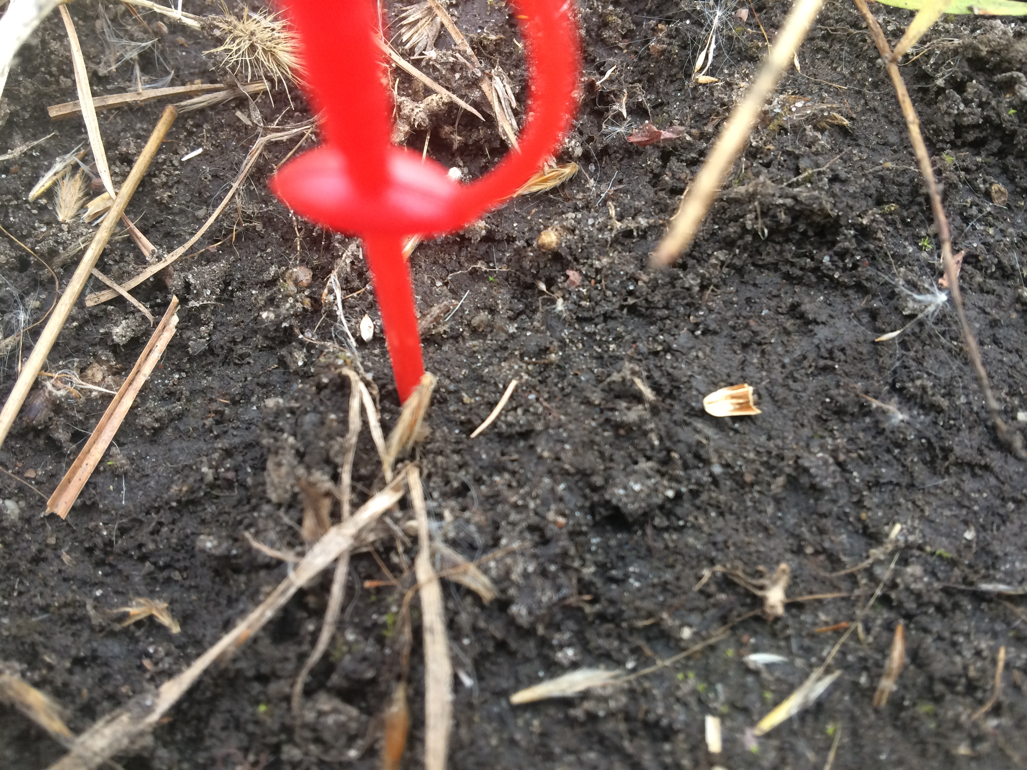
It was a dry and unseasonably warm day. This is lucky because there was 10 inches of snow where the plot is located a week and a half earlier. I was able to convince Matthew and Gooseberry to come along to help. Matthew was extremely helpful, but Goose mostly ate deer poop all day and threw up on the way home. Very yucky! To set up for planting, I staked to the end points for the rows we were planting, set up a meter tape, and then staked to and placed pin flags at positions every two meters along the rows. I started by placing pin flags every meter, but this was time consuming and a pin flag every two meters gave us a sufficient reference point for each meter.
We liked breaking the actual planting into two steps, and working in a pair, because it meant that we had fewer items to fumble around with and it was easy to catch and fix each other’s mistakes, such as accidentally skipping positions. I do not believe we made any actual goofs, which is a first for me with planting! For the first step, one person cleared the duff, and the other placed the corresponding vial. For the second, one person placed the achene and collected the vial, while the other placed the toothpick and carried the clipboard, making any notes, e.g., if the achene was planted a few cm off the row to avoid placing it on a rock or in bunchgrass. The first step took about 10-12 minutes per 50 positions. The second took about 8-10 minutes per 50 positions. We set the achenes on top of the soil so that they had good contact with the soil, but weren’t buried. We finished around 4 PM and were grateful that we did not have to plant in the dark.
I hope the seeds have a good winter and I look forward to seeing them in the spring!