|
|
Randomization is a critical aspect of any experiment. In almost all cases, the population being studied is much too large to study every individual, so a sample of the population is studied with the assumption that trends and relationships seen in the sample are also present in the population as a whole. In order for this to be a good assumption, the sample must be completely random in order to eliminate any bias towards a specific type of individual.
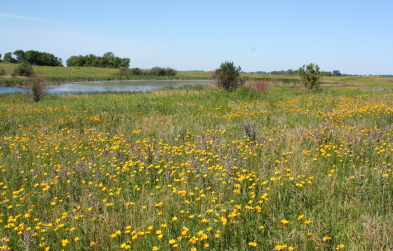
In an ideal world, all samples would be completely random, but this is not logistically possible in many cases. For example, at Staffanson Prairie Preserve, there are thousands of Echinacea that bloom every year. It would be a near impossibility to visit every single plant or even to select a completely random sample of plants within the preserve. For this reason, the Echinacea Project created a 10-meter wide transect through the preserve and studies the plants that fall within this transect. While this is not a truly random sample, it is able to approximate the range of conditions seen throughout the preserve.
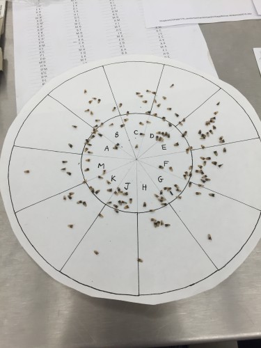
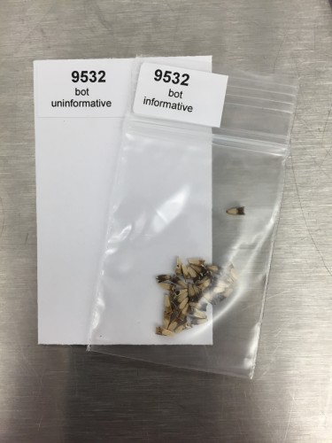
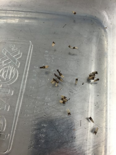
Another example of randomization is something I’ve been working on in the lab for the last week. Many of the heads contain several hundred achenes, so x-raying all of them to determine whether or not they contain a seed would be extremely time consuming and difficult. In order to simplify the process, I am randomly selecting 1/6th of the achenes from each head in order to estimate seed set for each head. While this will not give me the exact seed set, it will give me a very good approximation that will be sufficient for our analyses. Pictures of the randomization process are shown below—achenes are randomly dispersed on a wheel divided into twelve labeled sections of equal size. Next, two letters are selected from a list of random letters, and the achenes that fall within these sections are selected to be x-rayed.
 Achenes on the randomization wheel Randomized achenes–labeled and ready for x-raying
Katherine Muller’s paper “Echinacea angustifolia and its specialist ant-tended aphid: a multi-year study of manipulated and naturally-occurring aphid infestation” was selected by the Editors at Ecological Entomology as the most interesting paper in the current issue (41:1). This means that her paper will be highlighted on the Journal’s website and made Open Access for the next two months, along with a summary of the paper and an image of the ants attending the aphids.
Congratulations, Katherine! This paper was based on Katherine’s MS thesis in the Plant Biology and Conservation graduate program at Northwestern University. Katherine is now in a Ph.D. program at the University of Minnesota.
Here’s the text that is on the Journal’s main page …
Aphid abundance was manipulated on the perennial coneflower Echinacea angustifolia, which hosts a specialist aphid (Aphis echinaceae) tended by ants. Both have undergone extensive habitat loss and fragmentation. Aphids did not harm host performance after two years, though they did accelerate seasonal senescence. This experiment found a negative association between aphids and other herbivore damage, suggesting ant protection. However, observations showed the opposite trend, with larger plants more likely to have aphid infestation and leaf damage. The results suggest plant size drives foliar herbivory more than aphid infestation.
The paper was co-authored by Stuart Wagenius, Katherine’s MS adviser.
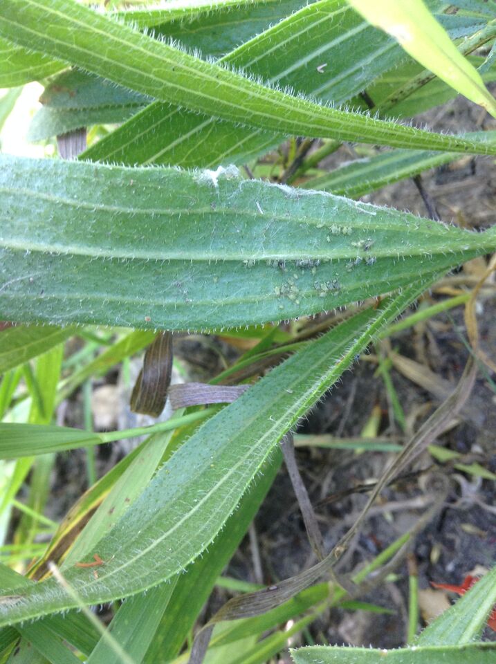
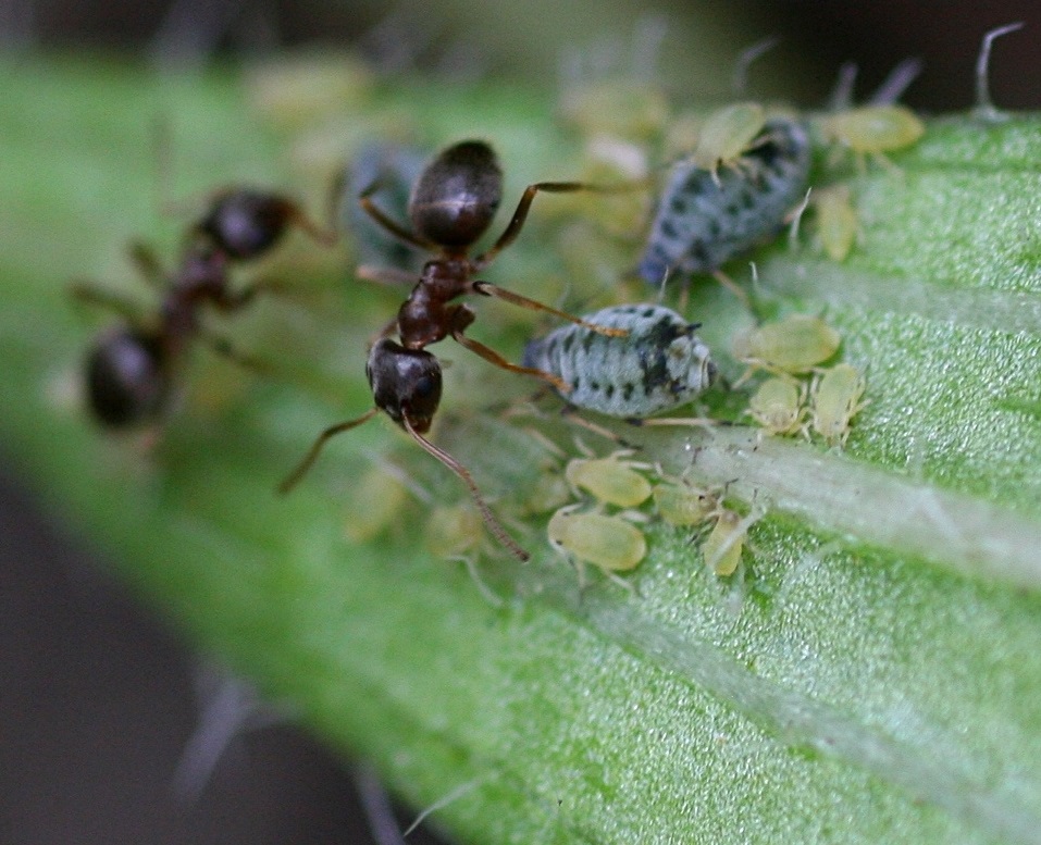
 Here are some of those cute little aphids!  This collection plant had some of the most aphids we’ve seen yet in one place! Specialist aphids, Aphis echinaceae, on a head of Echinacea angustifolia  Ants tending Aphis echinaceae
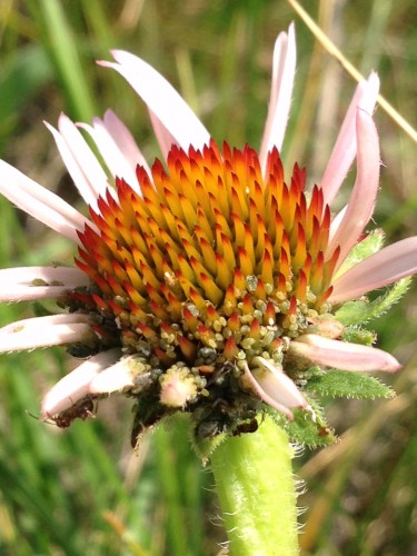
For the past three weeks, I’ve been hard at work collecting the achenes from Echinacea heads that were collected last summer from Staffanson Prairie Preserve. A little bit of Echinacea anatomy to give you a better idea of what I’m talking about: each head typically consists of 100 to several hundred small flowers or florets. After the head has matured and the florets have finished blooming, every flower produces one fruit, known as an achene, regardless of whether or not it was fertilized. Back at the lab, we clean all the achenes off the heads in order to count them and determine whether or not they contain a viable seed.
An intact head Achenes In addition to cleaning the heads, I have also been separating the achenes by where on the head they were located. The florets bloom row-by-row starting from the base of the head and working their way up, so we know that the florets at the bottom bloomed first and the ones at the top bloomed last. Looking at reproductive success via seed set on the top, middle, or bottom of each head will thus give an indication of how the mating scene and pollen availability changed over the course of the mating season.
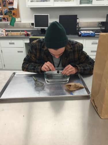
Hard at work cleaning a head Cleaning the heads is the first step in determining seed set, the primary measure of reproductive success I’ll be using for this project. Seed set is defined as the proportion of seeds that were successfully fertilized, and this number can range from zero to nearly 100%. While there are many reasons that fertilization may have failed, the primary reason is most likely a lack of compatible pollen. Now that all the achenes have been removed from the heads, I can determine what proportion of achenes on each head contains an embryo using x-ray. I’ll go into more depth about the x-raying process in another post.
In 2015, we continued the study of mating compatibility in the remnants that began in 2014. This experiment is designed to assess population level compatibility and to investigate whether difference in flowering phenology and distance between plants predict whether or not a cross will be compatible. We do this by randomly selecting focal plants from remnant populations and then choosing pollen donors which are representative of the ‘extremes’ of these variables–early flowering, late flowering, nearest to focal plant, and furthest from the focal plant.
 Bracts are painted to identify the pollen donor for each style of the focal plant that is being crossed This past summer we conducted this study in six of our largest remnant populations with approximately ten focal plants at each for a total of 228 pairwise crosses. Occasionally we were unable to collect pollen from the most ‘extreme’ individuals because they flowered asynchronously with the focal plant, and in those cases we chose the most ‘extreme’ individual available. Excluding all other pollinators, we performed hand-crosses between the focal plants and their pollen donors and assessed style persistence the following day to evaluate the compatibility of each cross.
Read more posts about this experiment here.
Start year: 2014
Location: large remnant populations
Overlaps with: comprehensive compatibility
Products: The 2015 data from this experiment has been combined with the 2014 dataset and awaits analysis.
Team members who have worked on this project include: Danny Hanson (2015), Amy Waananen (2015), and Claire Ellwanger (2014). Flog posts authored by these team members may provide additional detail about day-to-day activities associated with this experiment.
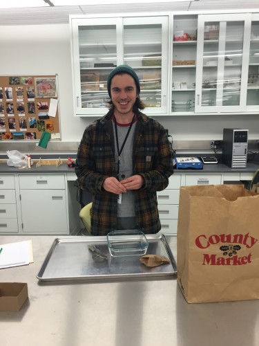
I’ve been helping out around the lab since the fall, but this is my first post on the Flog, so I’ll go ahead and introduce myself. I’m Gordon, and I’m a senior at Northwestern University studying Environmental Science and Chemistry. I have the awesome opportunity to conduct an independent study here at The Echinacea Project—not only will I learn research techniques and scientific writing skills, but I’m also able to get class credit for my research, allowing me to devote more time to the project.
Me with one of the many heads I’ve dissected
The main focus of my research is how fires affect the reproductive success of Echinacea. The existing scientific literature suggests that fires (or a lack thereof) redistribute resource availability, giving a survival advantage to certain species of plants. For example, a fire can burn tall prairie grasses to the ground, allowing shorter plants to access sunlight and contributing to their survival. In areas where prairie fires are suppressed, which includes many locations where prairie remnants exist today, it is thought that plants that benefit from fires will become scarcer. However, there is scant scientific literature regarding how fires influence the reproductive success of prairie plants.
At Staffanson Prairie Preserve, prescribed burns are conducted every five years, providing an ideal setting in which to conduct this observational study. I will be examining at plants that flowered both in 2015 (a non-burn year) and in a previous burn year. By comparing their reproductive success in both the burn year and non-burn year, I hope to gain an understanding of what influence fires may have on Echinacea reproduction. The measures I will use to study reproductive success will include: achene count, which indicates resource availability and reproductive effort; style persistence, which measures the pollen availability and limitation; seed set, which measures the success rate of seed production; and fecundity, which serves as an indication of total reproductive success.
Stay tuned for weekly updates about my procedure and progress over the next several months!
Over the course of four Wednesdays spread throughout November and October, we in the Echinacea lab were fortunate enough to have two students from Lake Forest College’s plant biology course. These students, Daniel and Kyle, looked at this year’s (2015) flowering plants that were in the aphid addition and exclusion experiment. They dissected, scanned, counted, and x-rayed the seed heads to determine seed set in these plants then made a poster and did a presentation for their class. It was wonderful to have them here and their contribution to the Echinacea Project will be very useful as we move on with the aphid addition and exclusion experiment.
You can find their poster here.
Read Ben’s Lee’s report and look at his map about pollinator habitat in Echinacea land.
This summer, Gina Hatch and Abby VanKempen continued a project examining the effects of aphid herbivory on Echinacea angustifolia survival and fitness. This year they found 70 of the original 100 study plants (33 addition and 37 exclusion). Starting July 14th going until August 20th, Abby and Gina visited plants twice each week for a total of 12 visits per plant. On each visit, the plant received its treatment: either adding aphids from other plants if it was in the addition group or removing all aphids if it was in the exclusion group. At the end of the summer, Abby and Gina used the number of leaves with chew marks and holes (signs of foliar herbivory) to quantify herbivory. There was not a significant difference in herbivory between the two treatment groups, where herbivory was measured as the proportion of damaged leaves (p = 0.74). On September 14th and October 15th, Ali Hall took measurements of senescence including number of brown and purple basal and cauline leaves. These have not yet been incorporated into an analysis.
Read more posts about this experiment here.
Start year: 2011
Location: P1
Overlaps with: Phenology and fitness in P1
Products: Fitness measurements were collected during our annual assessment of fitness in P1. A list of focal plants and addition/exclusion datasheets are located in Gina Hatch’s Dropbox folder and can be found here. Gina created a poster and presented at Carleton’s summer research symposium and her poster can be found here. Abby plans to present at the Elbow Lake Library. The senescence data can be found here.
Gina made a poster for Carleton’s summer research symposium. The symposium happened a while ago but you can relive the experience by looking at her poster!
Effects of the specialist aphid, Aphis echinaceae, on overall herbivory of Echinacea angustifolia
You can find it here.
For her RET project, Lea gathered data to study the relationship between flowering density and seed set. She worked at Staffanson Prairie Preserve, which appears to have higher flowering density in burn years than non-burn years. This year, 2015, was a non-burn year. Lea and Team Echinacea kept track of the style persistence of about 50 individuals for which we have seed set information from prior burn years. These individuals were harvested and their achene count and seed set will be assessed in winter 2016 by Gordon Younkin, an undergraduate intern from Northwestern University. Gordon will work to build a model of seed set in Staffanson in a non-burn year and aims to compare this model to a burn year.

Site: Staffanson Prairie Preserve
Start year: 1996
Location: Staffanson Prairie Preserve
Overlaps with: phenology in remnants, phen for aii
Products: Lea is developing a dataset and lesson plan for high-school students to compare individual plants’ style persistence in burn years and non-burn years to test hypotheses about seed set in high- and low- flowering density. This lesson will introduce students to R and its use in data management and statistical analysis.
Read other flog posts about this experiment.
|
|