|
|
I successfully created a generalized linear model to describe reproductive success at Staffanson Prairie Preserve for the 2015 season. I started out with a model containing distance to the 3rd nearest neighbor, flowering start date, flowering duration, section of head from with the achene came, and all interactions between these main effects. In addition, I included both linear and quadratic terms for distance, start date, and duration. The purpose of including a quadratic term is to test for evidence of curvature in the relationship to seed set.
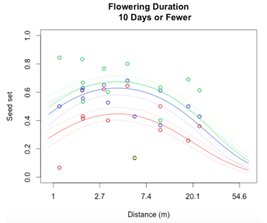
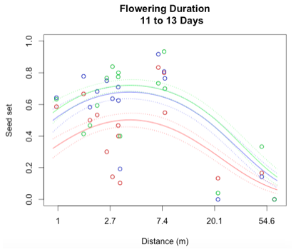
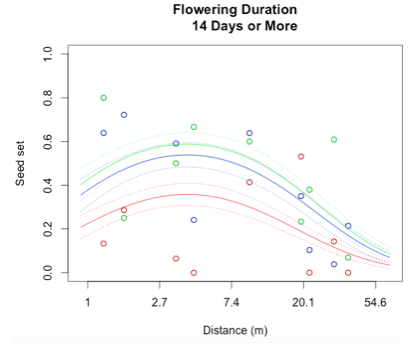
Through a process called backwards elimination, I removed all terms from the model that did not have a significant impact on reproductive success. The final model I came up with contained both linear and quadratic terms distance and start date, as well as the section of head. No interactions were found to be significant. In the plots below, the raw data are shown as points, and the predicted valued from the model are shown as curves. There are three plots of seed set as a function of distance, with the three plots representing low (10 days or fewer), mid (11-13 days), or high (14 days or more) flowering duration. The colors correspond to section of head, with red being top, blue is middle, and green is bottom.
  
While this is an observational study, so attributing causation would be inappropriate, it is helpful to think about why these relationships may exist. The general trend with increasing distance and spatial isolation is that seed set and reproductive success decrease. This is probably because isolated plants have fewer available mates or may be visited by fewer pollinators. However, the relationship is curved and plants in very densely populated areas also have diminished seed set. This may be caused by overcrowding and competition between plants for pollinators in areas of high population density.
Seed set has a similar peak at mid-duration of flowering. One explanation for this phenomenon is that plants that flower for a very short period of time co-flower with fewer potential mates, so a longer flowering time would maximize the number of compatible mates flowering at the same time. However, it is also known that extended flowering can be a sign that the head has not been receiving sufficient pollen, explaining the negative relationship between duration and seed set seen at higher durations.
In the future, this model will be compared to similar models from previous years during which Staffanson underwent controlled burns. Any differences seen between the models may be indicative of how the mating scene changes during the year after a burn.
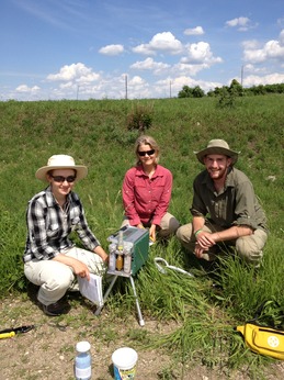
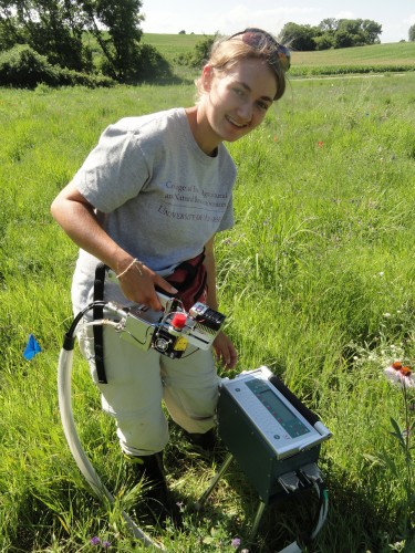
 Reina, Pamela, and Mike with the photosynthesis machine used in Kittelson et al. (2015) In 2015, we continued to study the effects of inbreeding on Echinacea angustifolia fitness. This experiment was planted in 2006 where each plant was produced from one of three cross types: between maternal half siblings; between plants originating from the same remnant, but not sharing a maternal parent; and between individuals from different remnants. We continued to measure fitness and flowering phenology in these plants.
This year, of the original 1443 plants in INB2, 561 were still alive. Of the plants that were alive this year, 8.3% were flowering and 76.3% have never flowered – we’re still waiting! Among the plants that were flowering, mean head count was 1.53 heads, with a maximum of five heads.
Read more posts about this experiment here.
Start year: 2006
Location: Experimental plot 1
Overlaps with: Phenology and fitness in P1
Products: Fitness measurements were collected during our annual assessment of fitness in P1.
The following paper was published in summer 2015 based on fieldwork conducted in 2013.
Kittelson, P., S. Wagenius, R. Nielsen, S. Qazi, M. Howe, G. Kiefer, and R. G. Shaw. 2015. Leaf functional traits, herbivory, and genetic diversity in Echinacea: Implications for fragmented populations. Ecology 96:1877–1886. PDF
With all of my data collected and visualized for the heads from Staffanson Prairie Preserve from 2015, it is now time to start with some initial data analysis. As I mentioned in my last post, I will be using R for all of my analyses, taking advantage of skills I learned in Stuart’s class at Northwestern this quarter. I will be creating statistical models based on the data to look for relationships between variables that may influence mate availability and reproductive success. The variables I am specifically looking at are:
- Distance to the kth nearest flowering neighbor. This is a measure of spatial isolation, with greater distance indicating greater isolation. Stuart has found a significant relationship between distance and reproductive success in Echinacea previously (that study can be found here: https://echinaceaproject.org/pub/wagenius2006.pdf)
- Start date and flowering duration. Flowering phenology, the timing and duration of flowering, is perhaps more important than spatial isolation in determining availability of compatible mates. If two plants are very close in space, but they do not flower at the same time, there is no possibility for mating. Previous data has shown that plants flowering earlier in the season have higher reproductive success (https://echinaceaproject.org/pub/isonAndWagenius2014.pdf)
- Section of head from which the achene originated. Because florets at the base Echinacea heads begin flowering first, and the ones at the top flower last, it is possible to examine how reproductive success, and thus the mating scene, differ for a single head across time. The bottom 30 achenes, the middle achenes, and the top 30 achenes are separated to represent the beginning, middle, and end of the timing of flowering.
- Seed set, or proportion of achenes that contain a seed, will be used to quantify reproductive success. This will be the that the model I create will try to predict using the variables I listed above.
In order to create a model, I will be using a technique known as backwards elimination as described in Statistics: An Introduction Using R (Crawley 2015). I will start by creating a statistical model containing my response variable (seed set), and all of my explanatory or predictive variables (isolation, phenology, section of head), along with all interactive effects between the explanatory variables. I will then eliminate a single predictor or interaction at a time and perform an analysis of deviance to determine whether or not that predictor was important to the predictive value of the model. If it is important, I will leave it in, but if it’s not, I will take it out. This process continues until all predictors and interactions left in the model have a significant effect on the response. This model, known as the minimal adequate model, is the simplest model that still includes all important variables.
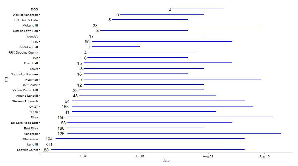
Beginning in 1996, Team Echinacea has monitored the flowering phenology of Echinacea angustifolia in remnant populations around Solem Township. The number of populations and plants we visit has varied over the years; a summary of which populations were monitored in each year can be found at this link. In 2015, we monitored phenology of 1763 heads on 1384 plants at 27 remnant populations. Whew! That is about 400 more flowering individuals than in 2014 although we monitored the same populations. Populations with big increases in numbers of flowering individuals from last year include Aanenson, East Riley, Landfill, and On 27. At each population, we identify all flowering individuals and track their development over the course of the season, gathering data on start and end dates of flowering for every individual. Flowering began at Loeffler’s Corner on June 23rd and ended at Aanenson on August 19th. We will use this data to describe temporal flowering patterns within and among remnants and relate this to potential for successful mating in populations.
 Blue line segments indicate the period of time that at least one individual was flowering at each population. The numbers to the left of the lines indicate the number of individuals that flowered from each population in 2015. Click to enlarge! Look here to read previous flog posts about this experiment.
Start year: 1996
Locations: roadsides, railroad rights of way, and nature preserves in and near Solem Township, MN
Overlaps with: mating compatibility in remnants, demography in remnants, phenology in experimental plots
Team members who have worked specifically on this project include: Amber Zahler (2011), Kelly Kapsar (2012), and Sarah Baker (2013), although gathering phenology data was a whole team effort in 2014 and 2015. Flog posts authored by Kelly, Amber, and other team members may provide additional details about day-to-day activities associated with our flowering phenology monitoring project.
Every year we keep track of flowering phenology in our main experimental plots, exPt1 and exPt2. Summer 2015 was a big year of flowering in both plots, especially in exPt2, where 1233 heads flowered between July 4th and August 26th. ExPt2 was designed especially to study phenology—you can read more about the team’s monitoring of phenology in the 2015 heritability of phenology project status update.
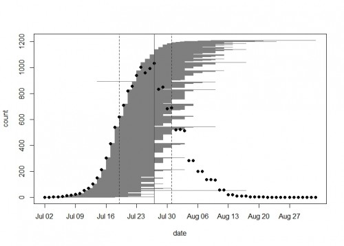
In exPt1, we kept track of 1212 heads on 649 plants (we left out the qGen_a ‘big batch’ cohort). The first head began shedding pollen on July 2nd and the latest bloomer shed pollen on September 2nd. Peak date in exPt 1 was on July 27th when there were 1034 heads flowering. At the end of the season we harvested the heads and brought them back to the lab, where we will count fruits (achenes) and assess seed set.
Read previous posts about this experiment.
 A plot of the 2015 flowering schedule in experimental plot 1 made with the brand new R package mateable–available now on CRAN! Each horizontal gray line segment on this plot represents the flowering time of one head. From bottom to top they are sorted by start day. Black dots show the number of heads in flower on each day. The vertical lines show the peak day (solid) and the days when half of the plants have started flowering and half have ended (dashed).
Start year: 2005
Location: Experimental plots 1 and 2
Overlaps with: Heritability of flowering time, common garden experiment, phenology in the remnants
Products:
These papers report on investigations of flowering phenology of individuals in experimental plot 1 in 2005, 2006, and 2007:
- Ison, J.L., and S. Wagenius. 2014. Both flowering time and spatial isolation affect reproduction in Echinacea angustifolia. Journal of Ecology 102: 920–929. PDF
- Ison, J.L., S. Wagenius, D. Reitz., M.V. Ashley. 2014. Mating between Echinacea angustifolia (Asteraceae) individuals increases with their flowering synchrony and spatial proximity. American Journal of Botany 101: 180-189. PDF
Taylor presented a poster of her summer research on fitness of native, non-native, and hybrid Echinacea plants at the Tennessee Louis Stokes Alliance for Minority Participation Conference. The meeting was held February 25-26, 2016 at the University of Tennessee-Knoxville. Taylor was awarded 3rd place in Science Poster Presentation category. Yay, Taylor!
Now that I’ve finished collecting data from the Echinacea heads collected from Staffanson Prairie Preserve in 2015, I am able to start doing some data analysis. While the ultimate goal is to compare the data from 2015, a non-burn year, to previous burn years, I first want to come to a good understanding of what reproductive success looked like in 2015.
For all of the analyses I will be doing, I am using computer software called R. R is a very flexible program that allows you to employ a wide range of graphical and statistical techniques including modeling, running tests, and clustering. Although R does have a somewhat steep learning curve, I have been learning many useful techniques in Stuart’s class on R at Northwestern and am confident in my ability to properly analyze the data I have collected.
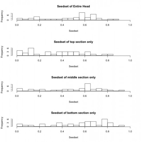
The histograms below show seedset, which is the proportion of achenes that contain a seed and can range from zero to one, for the entire head, as well as for the top, middle, and bottom sections of each head. For the entire head, the sample has a range from 0 to 0.86, with a mean of 0.48 and a median of 0.57. While the middle and bottom portions of the head had similar seedsets, the top portions of each head appear to have lower seed set on average when compared to the rest of the head. This is consistent with the findings of previous years and suggests that florets that are receptive to pollen later in the season may have diminished reproductive success.

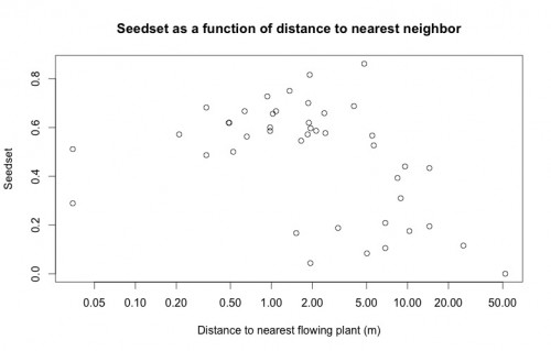
An important variable in Echinacea reproduction, spatial isolation, is modeled in the below plot as a predictor of seedset. This plot highlights the importance of doing a careful visual exploratory data analysis before diving into more complicated statistical analyses. While there does appear to be the expected inverse relationship between seedset and spatial isolation, upon looking at this plot Stuart was immediately able to tell me that the two points on the left of the plot are the result of erroneous data. None of the plants have a nearest neighbor less than 5 cm away, so there must have been an error either in data entry or during the recording of GPS coordinates. Because we have records for the correct GPS coordinates of every plant, this will be a very easy error to fix, but had Stuart not looked closely at this plot, I may have done the entire analysis with incorrect data.

 The functional trait machine used in the Kittelson et al. paper. In 2015, we continued to study the effects of inbreeding on Echinacea angustifolia fitness. This experiment was planted in 2001 where each plant was produced from one of three cross types, depending on the relatedness of the parents: between maternal half siblings; between plants from the same remnant, but not sharing a maternal or paternal parent; and between individuals from different remnants. We continued to measure fitness and flowering phenology in these plants.
This year, of the original 557 plants in INB1, 157 were still alive. Of the plants that were alive this year, 23.4% were flowering and 24.9% have never flowered. Among the plants that were flowering, average head counts was 2, with a maximum of six heads.
Read previous posts about this experiment.
Start year: 2001
Location: Experimental plot 1
Overlaps with: Phenology and fitness in P1
Products:The team collected fitness measurements during our annual assessment of fitness in all plants in P1.
The below papers were published in summer 2015:
Kittelson, P., S. Wagenius, R. Nielsen, S. Qazi, M. Howe, G. Kiefer, and R. G. Shaw. 2015. Leaf functional traits, herbivory, and genetic diversity in Echinacea: Implications for fragmented populations. Ecology 96:1877–1886. PDF
Shaw, R. G., S. Wagenius and C. J. Geyer. 2015. The susceptibility of Echinacea angustifolia to a specialist aphid: eco-evolutionary perspective on genotypic variation and demographic consequences. Journal of Ecology 103:809-818. PDF
The oldest Echinacea plants in experimental plot 1 will turn 20 this year. They are part of the 1996 cohort, which was planted in a common garden experiment designed to study differences between remnant populations and assess life history traits as they grew. Stuart sampled about 650 seeds (achenes) from eight remnant populations in and near Solem Township, representing the range of modern prairie habitat from small patches along roadsides to a large nature preserve. In 1996, he transplanted seedlings on a 1m x 1m grid, randomly assigning the location of each individual.
Every year, members of Team Echinacea assess survival and measure plant growth and fitness traits including plant status (whether it is flowering or basal), plant height, leaf count, and number of flowering heads. We harvest all flowering heads in the fall and obtain their achene count and seed set in the lab.
Of the original 650 individuals, 304 were alive in 2015. This year, 136 individuals from the 1996 cohort were flowering with a total of 303 heads. At present, these heads are in the lab where they await processing to find their achene count and seed set. We used 31 plants (45 flowering heads) from the 1996 cohort as maternal plants in crosses for the most recent heritability of fitness experiment (qGen3). We also used five plants from the 1996 cohort (8 heads total) as part of the pollen exclusion and addition experiment. We covered their heads with pollinator exclusion bags for the duration of the season.
Read more posts about this experiment.
 Stuart passes out pollen to Gina and Ben for crosses between 1996 cohort plants in the qGen3 experiment Start year: 1996
Location: Experimental plot 1
Overlaps with: phenology in experimental plots, qGen3, pollen addition/exclusion
Products:
Much of the work I have been doing up to this point has been to determine a single number for each head—the proportion of all achenes on a given head that contain a fully formed seed, or seed set. This gives a good indication of how successful that plant was in terms of reproduction. The most likely reason that an achene does not contain a seed is that the flower did not receive compatible pollen, either due to a lack of mates or due to a limitation on the part of the pollinators.
In order to determine seed set, I need two numbers: the total number of achenes and the number of achenes containing an embryo. While the achenes could be counted by hand, this would be a tedious and error-prone process. Instead, the achenes were placed on a glass tray and scanned into the computer and counted digitally.
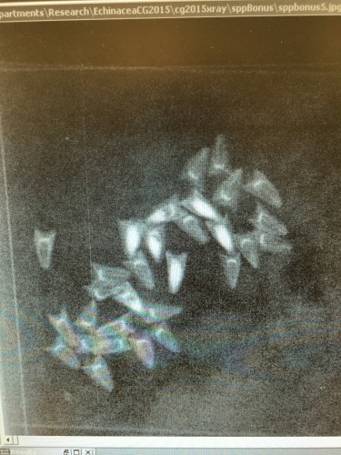
It is possible to determine whether or not an achene contains a seed by several methods. Germination experiments are useful because every achene that germinated certainly contained a seed, but they can be time-consuming and demand lots of attention and resources. Another possibility is to weigh the achenes. Heavier achenes are much more likely to contain a seed, and lighter achenes are most likely empty. We chose to use x-ray, which allows us to see directly inside of each achene. When achenes are x-rayed, empty achenes are barely visible while seeds show up as opaque. Ideally, all achenes could be easily categorized into “empty” or “full,” but some achenes are partially full, likely meaning they were initially fertilized but full seed growth was not entirely successful.
Together, these numbers are very important in allowing us to make inferences about what conditions are best for Echinacea reproduction.
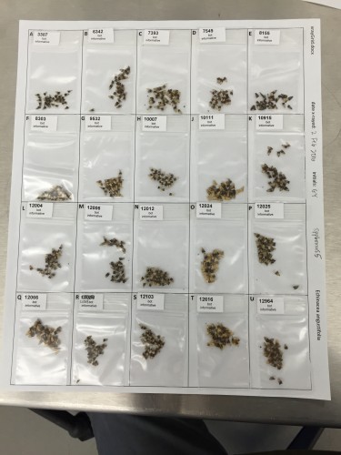
Randomized achenes ready to be x-rayed.
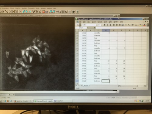
This is what x-rayed achenes look like. Achenes that contain a seed show up with a white oval in the center. Full, partial, and empty achenes are counted on the computer and entered into an spreadsheet.
|
|