I couldn’t make the Midwest Ecology and Evolution Conference, but I made a poster. It describes preliminary results from an aphid addition/exclusion experiment I conducted in the summer of 2011. Specifically, it examines the question of whether aphid infestation influences the presence of leaf damage by other herbivores.
|
||||
|
Hello everyone! This is Sebastian with another update on the x-ray machine. This post will discuss the various methods that can be used to determine the radiation dose of our x-ray machine. Below you will find my report on determining x-ray radiation doses.
Evaluating 3 methods for estimating radiation doses
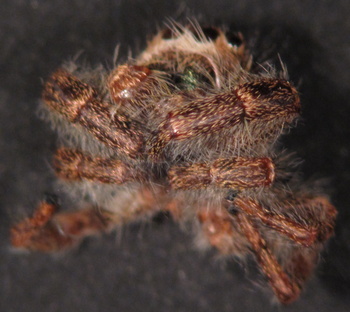
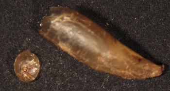
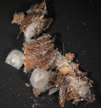
Introduction: Objectives: Methods: Results: Comparison between manufacturer data and web calculator: The web calculator: http://www.radprocalculator.com/XRay.aspx The information given by the manufacturer is given in the following documents: MX-20 mR Ouput versus time.pdf The professionals offer the solution of a dosimeter. Conclusion: Since the manufacture data is most reliable it is the clear choice to use. The manufacturer data covers more information, such as time, voltage, as well as unit conversions for other factors. Considering that more information is provided more variations to experiments can be made and the radiation does would still be available after simple unit conversions. The other option presented by professionals would be to use a dosimeter to directly measure the radiation dose. This option would be the easiest way out of the three options, and would cater more to a researcher’s specific setting. If a dosimeter is available to use I would make this device my choice for determining radiation dose. Hi everyone! Maria here. Sorry that I have not posted since the end of summer, but please rest assured that I’ve not run away with my Dichanthelium seeds, but have been working on them for the past -what? 6 months? A long and intimate relationship indeed. Brief summary of what has happened: I did a pilot germination & growth study using bulk Dichanthelium seeds. The results of germination study is nicely summarized in this poster that I presented at Midwest Ecology and Evolution Conference (MEEC) in Cincinnati 2 weekends ago(?). MEEC was fun and presenting (yapping about) my poster was a lot less nerve-wracking than I had expected: The seedlings are currently growing in the growth chamber at CBG. (There’s pictures in the poster of seedlings in agar and in plug trays!) I shall put up some more pictures sometime in the future. I should also post the R script I used to analyze data and produce the graphs on the flog – unfortunately don’t have the file on this computer. Right now I’m working on scarifying Dichanthelium seeds for my maternal lines growth and germination experiment (probably should explain in better detail later, likely in another poster). Other good news you might find interesting: If you have any questions about Dichanthelium or anything I talked about, you’re welcome to get in touch. My email is right under the entry title. Hello Project Echinacea Flog!,
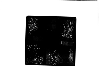
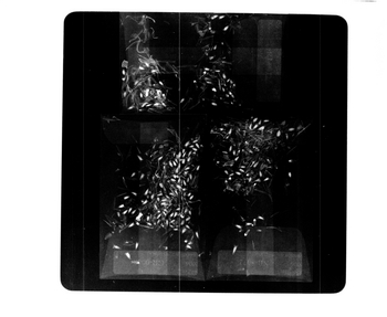
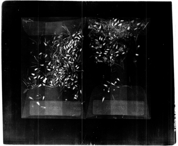
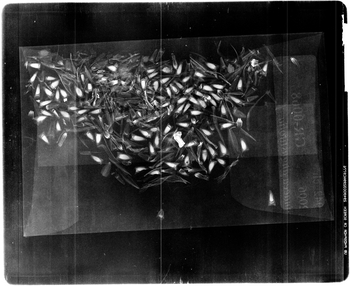
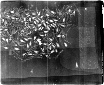
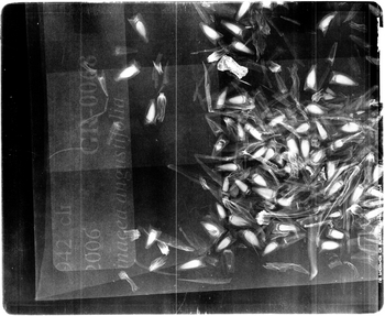
X-ray machine magnification Introduction: The population biology lab is trying to determine the best x-ray magnification to use for scanning Echinacea achenes. The criteria that constitute “best” are image quality and contrast, label legibility, and overall time and efficiency. Each magnification presents different advantages and disadvantages, some more prominent than others. The use of these x-rays can give a more definitive answer of whether an achene has been fertilized compared to achene weight. With this experiment I will evaluate the x-ray machine magnification levels and determine the best choices and ideally isolate one magnification setting that would be best. Objectives: 1. Obtain the best contrast quality possible for achenes Methods: I scanned batches of Echinacea achenes in envelopes under the 10 second and 18 kv setting on the x-ray machine at the varying magnifications (magnifications are 1:1; 1:1.5; 1:2; 1:3; 1:4; 1:5) and window level settings. After taking a number of images at each magnification and assigning the prescribed window level settings (see X-Ray Machine Protocol for Echinacea) I compared images side by side. I then documented similarities and differences, and pros and cons of each image on their own and in relation to the other images taken. Based on the resulting images and my notes, I determined what each magnification might be useful for. Finally, I choose two magnifications out of the six that I thought would be most useful, and then weighed the pros and cons of each one more heavily and made my final choice as to which magnification would probably be best. Results: 1:1 Magnification
At the 1:1 magnification the labels are hardly visible. The zooming in on this image would not do that much good because the image will become more pixilated. It is quite difficult to distinguish the achenes that are hollow and have not been germinated. Also, it is not possible to tell where the envelopes end or begin. The only real benefits of this setting are that four envelops can be scanned at a time and the achenes that have an embryo can be fairly easily counted. 1:1.5 Magnification
A magnification of 1:1.5 clearly does not show the greatest image. Although three envelopes can be captured in the image the labels are rather difficult to read and part of the third envelope gets cut off. The orientation of the envelopes is also a bit confusing and more laborious to set up. Positives of the image are that a large sample of achenes can be processed at a time. Another benefit is that after zooming in on the picture the achenes are easy to count and the visibility of germinated and non germinated achenes is fairly clear. 1:2 Magnification
The first benefit the 1:2 magnification has is that two envelopes can be scanned at a time. This benefit can double the speed of the scanning process. The extra space around the two envelopes can be use to include any smaller envelopes that may come inside the main envelope. The labels in this setting are still readable and the achenes show up nicely. The image needs to be zoomed in upon to provide a more accurate count of the achenes and to tell which have been germinated and which have not. If time is not of the essence, one of the magnification settings soon to follow would be recommended. 1:3 Magnification
The magnification setting of 1:3 is a good compromise between the previous settings and the settings to soon be discussed. This setting provides an image that encompasses a full envelope and leaves some room to spare. The extra room can be used for adding any small envelopes used to set aside certain achenes that may come inside the main envelope. The label in this image is fairly legible and every achene can be counted. It is also possible to determine which achenes have an embryo or are lacking an embryo. Furthermore, if the image is zoomed in upon it is possible to see any damage or defects of the achenes. The only issue with this magnification setting is that only one envelope can be scanned at a time, which makes the overall scanning process proceed at a slower tempo. 1:4 Magnification
A 1:4 magnification setting provides a fine image that shows both the label and the achenes clearly. From this magnification it is easy to count achenes, see any damage or defects of achenes, and tell whether achenes are hollow or have an embryo. Drawbacks to this setting are that the entirety of the envelope is not captured in the image, which leaves achenes not visible at the bottom or top of envelop that is cut off. Another obvious set back is that it is only possible to view one envelope at a time. This setting would be recommended to use if a close examination of the achenes is need, especially when trying to examine a greater number of achenes at a time. 1:5 Magnification
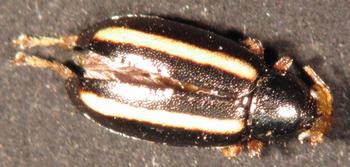
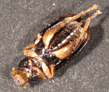
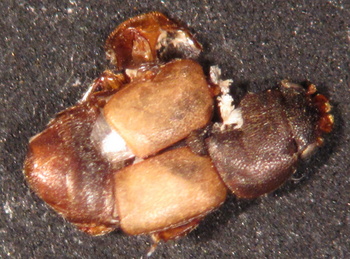
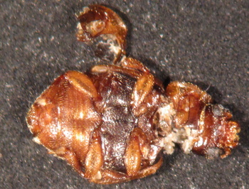
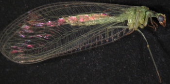
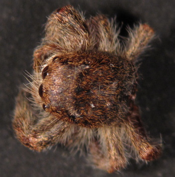
At a 1:5 magnification the clearest results are returned. Each achene can easily be counted, identified as hollow or full, and the label is clearly legible. This magnification is the highest magnification possible on this x-ray machine and is therefore the high-end extreme. The negative aspects of this magnification are that it is not possible to capture the entire envelope in the image. Unless all of the achenes are pushed towards the label there is no way of telling how many achenes may not be accounted for. As a result of not being able to fit one full envelop in the image it is not a far stretch of the mind to understand that capturing two envelopes at this magnification setting is out of the question and that only one envelope (or part of one). At this magnification, it would only be recommend to be used to examine certain achenes in order to inspect damage, shape, or any other anomaly that is being investigated. Conclusion: Considering all of the magnification settings, the top two would have to be 1:2 and 1:3. These levels have the most benefits out of all of the other settings without all of the negatives of the other settings. These two options are thus recommend for use. The question that presents itself is a matter of time and efficiency, and what setting is best to use. At the 1:2 setting, does the time saved by scanning two envelopes at a time out weigh the time it would take a person to zoom in on each envelope and count the achenes and determine which are germinated and which are not? At a 1:3 magnification, does the time to scan one envelope at a time and continually switch out samples negate the time it takes for a person to count the germinated and not germinated seeds without zooming in? After carefully considering the question of time and efficiency I conclude that the 1:2 magnification setting is indeed the best choice and the 1:3 setting the second best choice. The time it takes zoom in on one envelope to count the achenes and determine their germination states and then zoom out and zoom in to do the process over is shorter that the time it takes to scan one envelope at a time and be easily to count the achenes and determine the germination states without needing to zoom in. To zoom in and out and back in takes far less time than completely going through the image scanning process for individual envelopes. The time it takes for the media plate to go through the CR reader is what takes the longest and makes the 1:3 magnification the second best choice. All accounted for, the best magnification setting to use is 1:2 for time and efficiency sake. If time is not of the essence, then the 1:3 magnification setting would be the best option. The final ranking of all of the magnification settings would be: A.) 1:2 B.) 1:3 C.) 1:4 D.) 1:5 E.) 1:1.5 and F.) 1:1 respectively. This ranking and the best option may very based on the experiment being run, sample size, and what the object of inquiry is. For a general scanning to most efficiently count and determine germination states this ranking holds. If a different experiment is being conducted and or a different sample size or object of inquiry is at hand then the best setting to use should be determined as needed based on the pros and cons as listed in the previous pages. Hello Project Echinacea Flog!, Report: Appendix In the lab, we have found more insects, a spider, and a lot of web in the Echinacea heads we have been cleaning. The insects include another lacewing fly and two beetles that I cannot identify. I also found a hard shell that looks like a Syrphid fly pupal case. I have the web and the egg sacs clustered because of the amount that we tend to find in the lab. Unidentified Beetle No. 1: Unidentified Beetle No. 2: Lacewing Fly: Spider: Syrphid Fly Pupa Case: Spider Web Cluster: Here is the protocol that we plan to use for measuring in 2012: Here’s a link to the protocol that we used for measuring CG1 in 2011: In 2012 we plan to measure in “review mode” (as we did for CG2 in 2011) — all location records will be on the Visors with Status=”Staple” or “Skip” populated. We should not spend as much time searching for plants that have not been present for 3 or more years.This should speed up measuring. I’ll post the planned 2012 protocol next. Now that we’ve inventoried all the CG1 heads, I checked to see just how many we have. There were about 3009 twist-ties put out, and 119 heads were duds or missing, so our (estimated) total number of good heads is about 2890. CG2 had something like 140 heads, but we haven’t inventoried those yet. In a paper just published in PLoS ONE, Echinacea Project researchers show how habitat fragmentation may make plants more susceptible to aphid attacks. Aphid abundance early in the season is higher on inbred and outcrossed Echinacea angustifolia plants compared to regular plants. Elemental stoichiometry plays a role in this plant-herbivore interaction, but other genetically-based plant traits must also attract or encourage aphids. Ridley CE, Hangelbroek HH, Wagenius S, Stanton-Geddes J, Shaw RG, 2011 The effect of plant inbreeding and stoichiometry on interactions with herbivores in nature: Echinacea angustifolia and its specialist aphid. PLoS ONE 6(9): e24762. Available online at http://dx.plos.org/10.1371/ |
||||
|
© 2026 The Echinacea Project - All Rights Reserved - Log in Powered by WordPress & Atahualpa |
||||