|
|
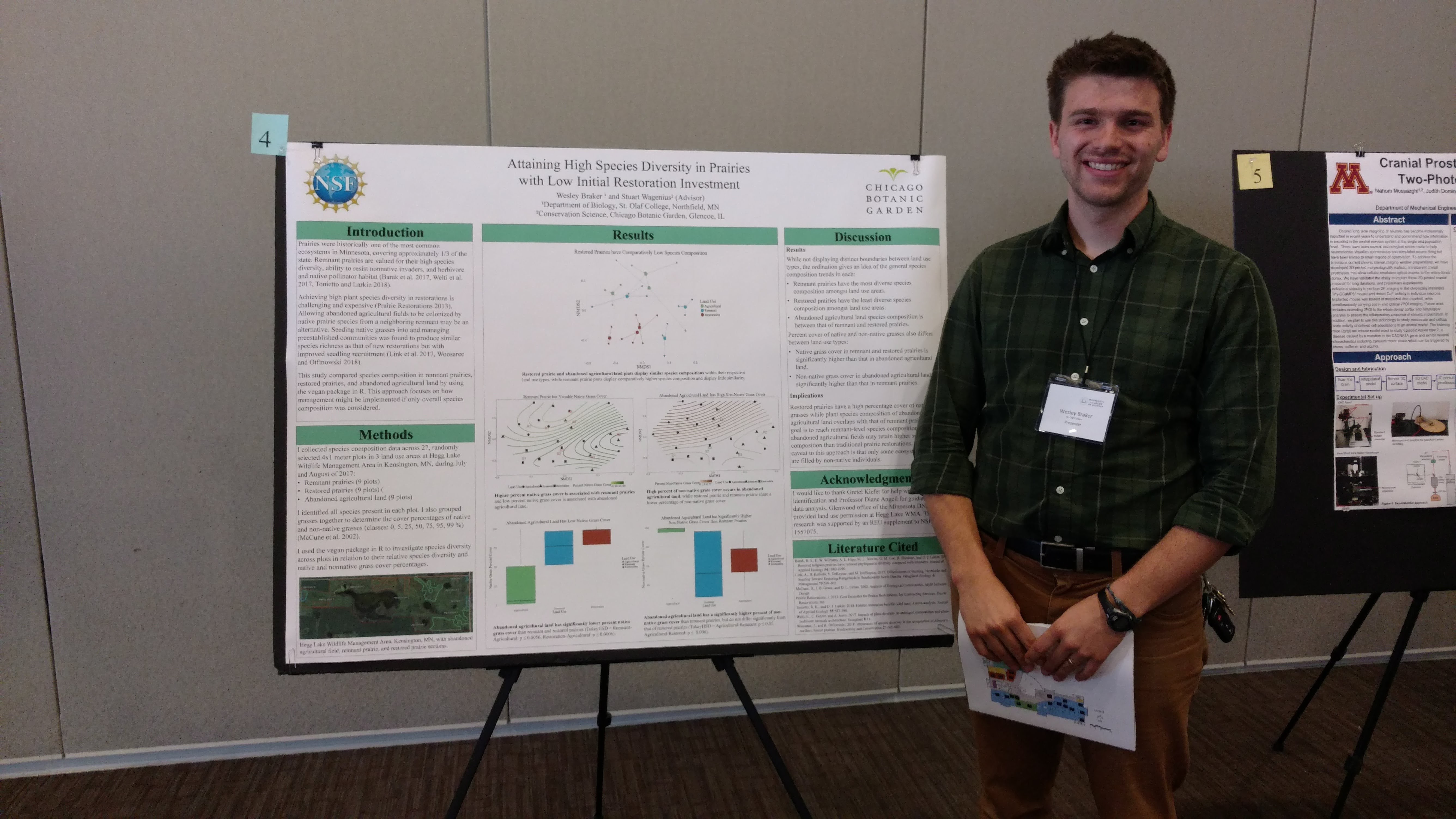
Wes presented the poster “Attaining high species diversity in prairies with low initial restoration investment” at the 85th Winchell Undergraduate Research Symposium & 31st MAS Annual Meeting with Stuart as co-author at the University of St. Thomas, St. Paul, MN on 21 April 2018. Here’s the poster.
Yay, Wes!
 Wes presents his poster.
Hi all! Stuart and I are in the process of figuring out the best way to edit our x-ray images of Echinacea achenes so that it is easy to classify them:
- Are all achenes (full and empty) visible?
- Is it easy to tell between full and empty achenes?
- Can achenes within clumps be identified individually?
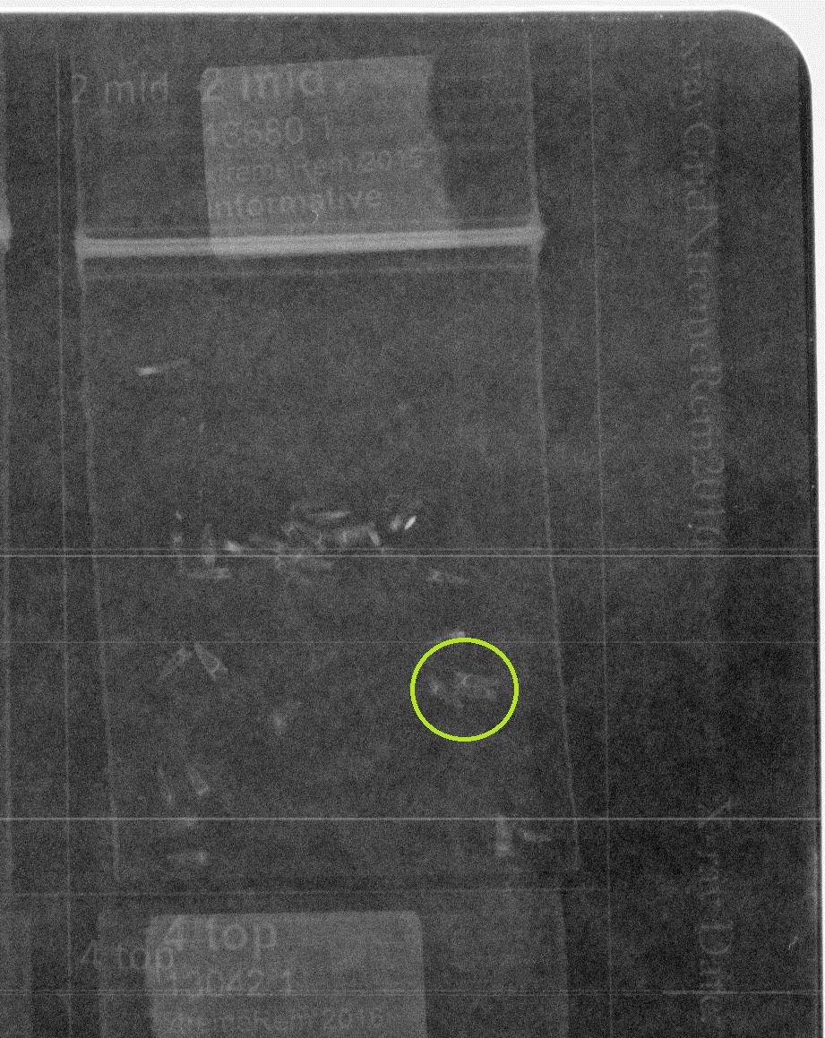
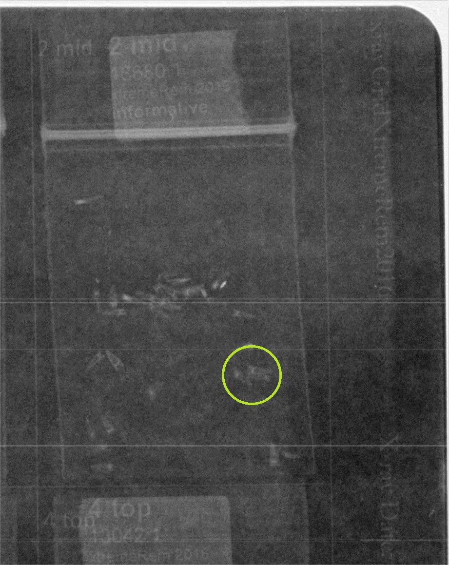
 Example x-ray image with achenes, before edited Here is an example of an x-ray image that is tricky to classify. All of these achenes are empty, so they are more translucent and harder to see. Also, many of these achenes are in clumps, so getting the correct count of empty achenes is a challenge.
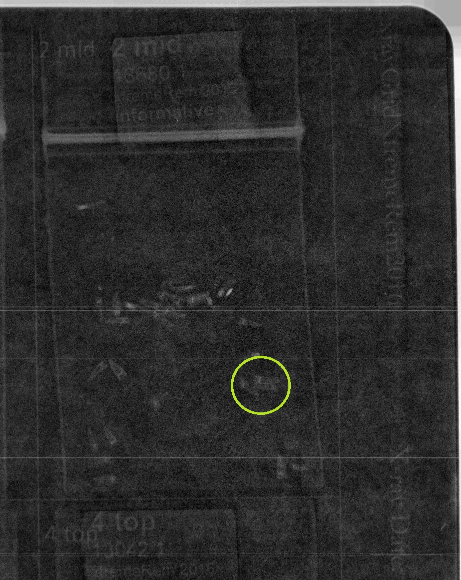
Example x-ray image before edits, with circled clump A single clump has been circled in green in this image. This clump has 3 empty achenes, but we want that to be more obvious. To edit our images, we have been working with the EBImage package in R. Here are a few examples.
Edited example #1 This edit is helpful because it makes the background darker so that it’s easier to pick out achenes. The 3 in the clump are still kind of hard to pick out, though. Here is the code we used:
library(EBImage)

x <- readImage('https://echinaceaproject.org/wp-content/uploads/2018/04/x2mid.jpg')
display(x)

kern = 2000*makeBrush(99, shape = 'Gaussian', sigma = 5)
display(whiteTopHat(x, kern))
This example is blurred a bit, which is helpful for seeing achenes in their entirety. This is the code we used:
library(EBImage)

x <- readImage('https://echinaceaproject.org/wp-content/uploads/2018/04/x2mid.jpg')
display(x)

display(gblur(x, sigma=0.8))
There are endless possibilities if using multiple EBImage functions on one image, and we are looking for some guidance. If you have experience with EBImage, what do you think are the best combinations of functions for reaching our goals? Thanks for the help!
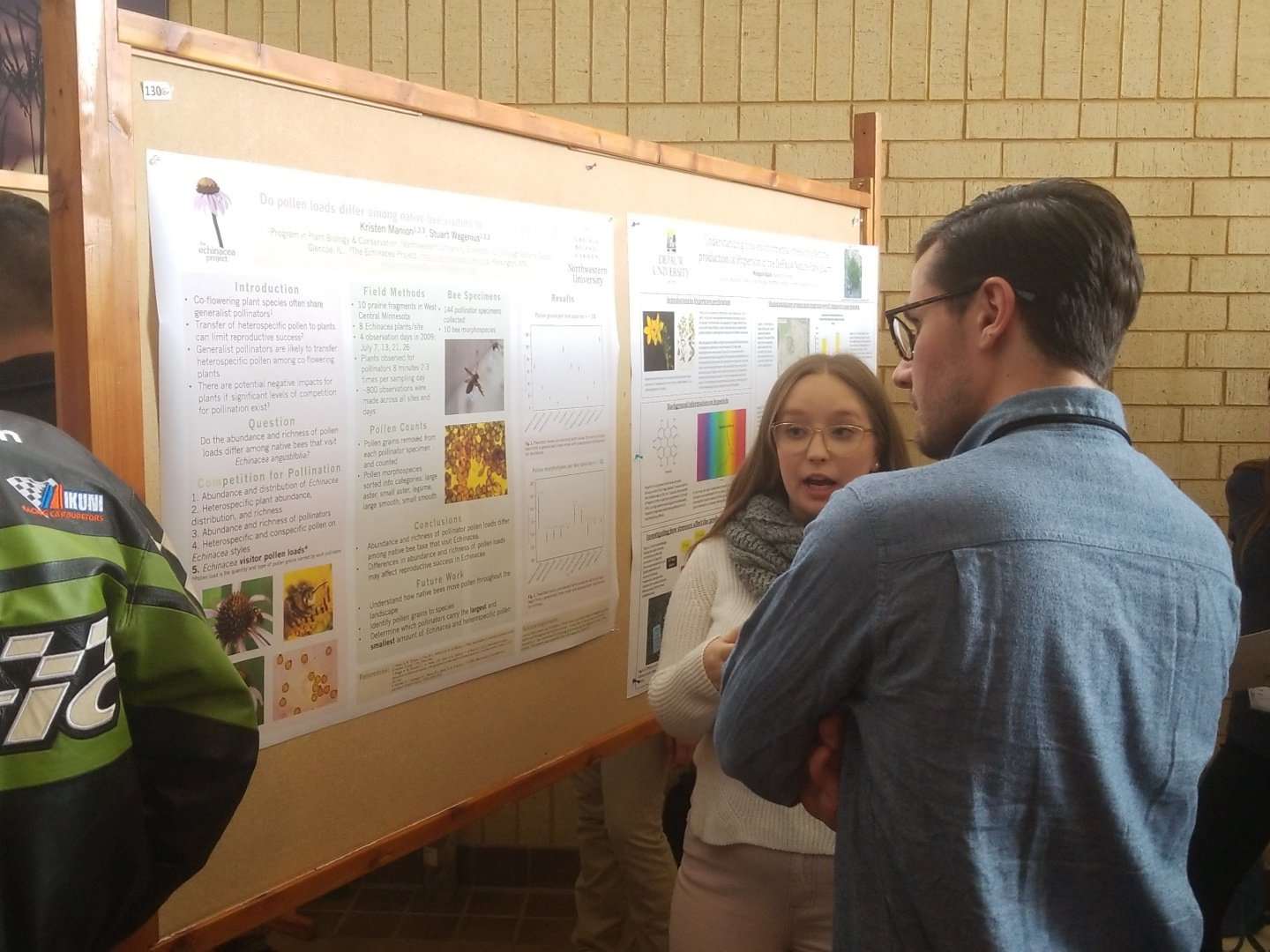
Hi everyone! Tracie, Kris (another PBC grad student), and I had a great time presenting this year at the Midwest Ecology and Evolution Conference in Kalamazoo, MI. Here’s a look at my poster that I presented about pollen on Echinacea as a part of the ongoing Floral Neighborhood Communities project:
 Do pollen loads differ among native bee visitors to Echinacea angustifolia? A picture of me presenting! MEEC 2018 was awesome! For any undergrad or graduate student interested in attending an inexpensive, regional conference I would highly recommend it. It was great to network with fellow graduate students and hear all about the great research ongoing here in the region!
It’s time to prepare annual reports to NSF for our two long-term awards through CBG & through UMN. The period covers 1 April 2017 through 31 March 2018. So, here’s a brief recap of activities from the past 12 months including the summer 2017 field season.
Last spring we were busy in the lab. Led by interns Amy & Scott, volunteer citizen scientists at the Chicago Botanic Garden started cleaning heads harvested in summer 2016 to count all of the achenes to generate a detailed and precise dataset of annual plant reproductive fitness. We were way behind because of the huge flowering year in 2015. We worked all fall & winter and we are in good shape now. Led by Tracie, we are cleaning 1148 heads harvested from plots in 2017, which we will finish over this summer.
Several undergraduate students have worked on projects in the lab, including Nicolette, Ashley, Marisol, Nina, Trevor, and now Danielle. They are all gaining experience, learning a lot, and contributing to science! Graduate students are hard at work too. Lea has analyzed all of her summer phenology data on Solidago & Liatris. Kristen is working on the bee collection from last summer with Mike. They are both making research plans for summer 2018.
Last December, we submitted a paper to Oikos titled “Pollinator-Mediated Mechanisms for Increased Reproductive Success in Early Flowering Plants.” We haven’t heard anything for 101 days & wonder if it has disappeared into a black hole.
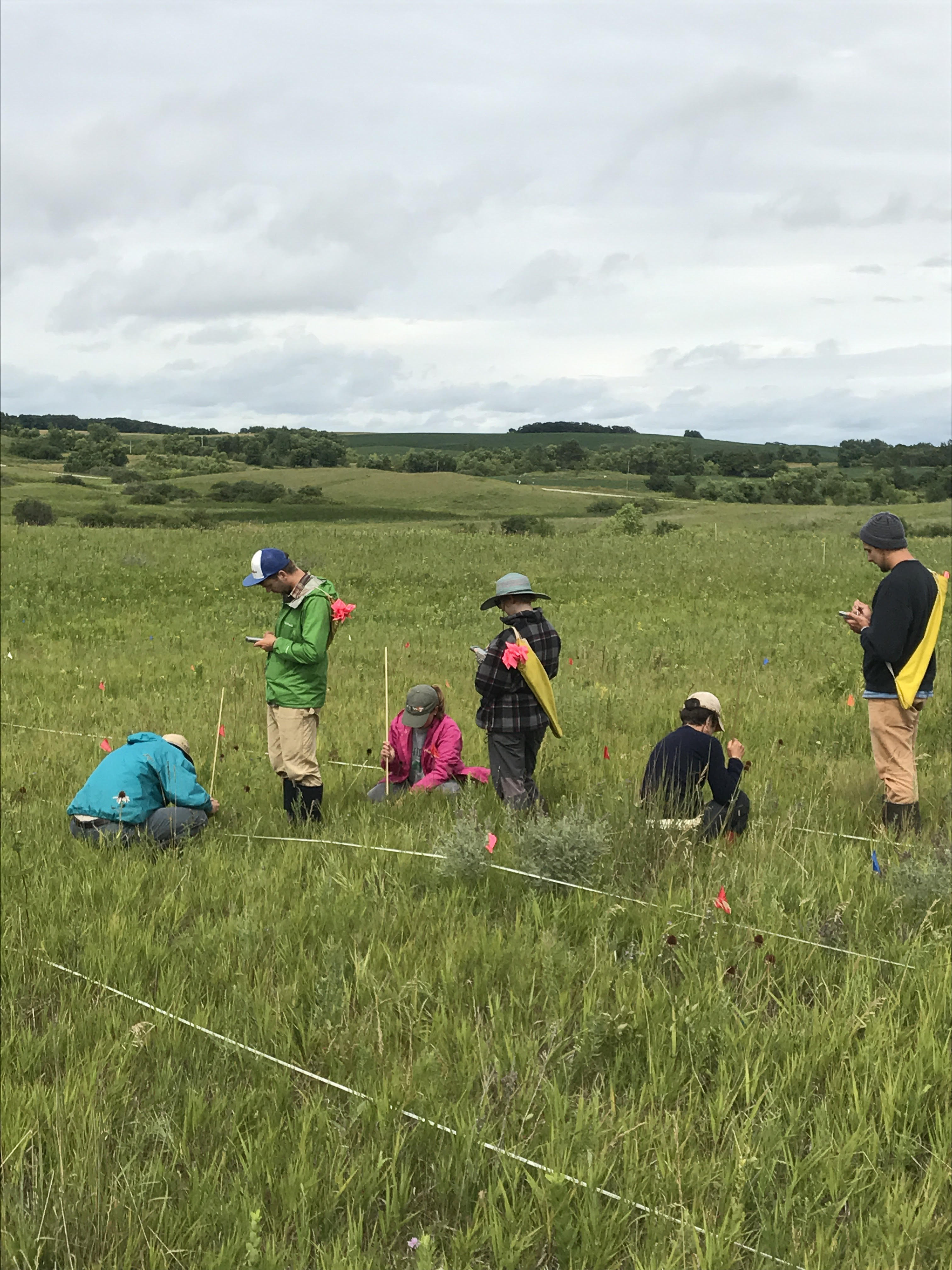
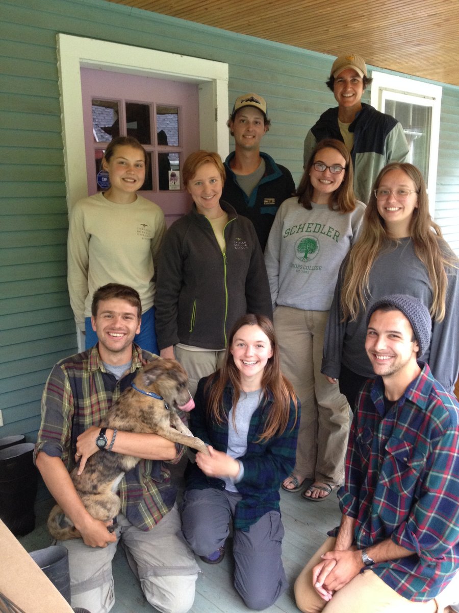
Our team accomplished a lot in summer 2017! The 2017 summer team, shown below, included three undergraduate students (Ashley, Will & Wes), a high-school student (Anna), two graduate students (Lea & Kristen), and two recent college grads (Tracie & Alex)–not to mention the usual suspects, Gretel, Ruth & Stuart. We summarized progress on many summer projects last fall & made flog posts. Here are links to the updates organized into six groups.
First, we measured survival, growth, and flowering effort of our model plant, Echinacea angustifolia, in several experimental plots. The earliest was established in 1996 and the most recent in 2015:
Second, we measure other traits in these plots, including flowering phenology. We also have some treatments, such as pollen addition and aphid addition, which we apply every year. Will has super-cool estimates of the heritability of flowering timing. He is polishing the manuscript and will submit it soon. Amy W. has a manuscript in review that quantifies reproductive synchrony in the 1996 cohort of plants. She estimated how much within-year synchrony (daily phenology) and among-year synchrony (annual flowering) contribute to long-term mating opportunities.
Third, we make observations of Echinacea plants in natural prairie remnants in our study area, including flowering phenology, survival, reproduction, and incidence of disease. Scott is investigating effects of fire on population growth rates in our remnants using a life-table response experiment approach. While she is on sabbatical, Amy D. is analyzing the seedling establishment dataset.
Fourth, we study plant species other than Echinacea angustifolia and we are very interested in pollinators, including native solitary bees.
Fifth, two REU participants worked on our Team last summer. Here are updates of their projects.
Sixth, we are worried about non-native Echinacea plants that are used in restorations and how they impact populations of the native Echinacea angustifolia. We have several ongoing experiments that investigate a population of Echinacea pallida introduced within our study area.
 The Team from summer 2017
Hello, Nina here! These past few months, I was an extern with the Echinacea project, looking specifically at data collected last summer about Echinacea success and surrounding plant diversity. My findings are summarized in the report that I’ve attached here.
Anna and Will decapitate a plant. It’s Echinacea pallida which is not native to Minnesota. Echinacea pallida is an Echinacea species that is not native to Minnesota. In July 2017, we identified 100 flowering E. pallida plants with 222 heads that were planted in a restoration at Hegg Lake WMA. Every year for the past several years, we have visited the E. pallida plants, taken phenology data, and chopped off their heads. On July 7, 2017 when we collected the data, the maximum male row was 19, meaning flowering started about 19 days earlier–June 18, 2017. E. angustifolia in the remnants started flowering on June 24, about a week later. 17 of the 222 E. pallida heads were still buds on 7 July, so these plants would have continued flowering for awhile.
We went back to check if we missed any heads on 31 August and found two. They were done flowering, but hadn’t dropped seeds.
Start year: 2011
Location: Hegg Lake WMA restoration
Overlaps with: Echinacea hybrids (exPt6, exPt7, exPt9), flowering phenology in remnants
Physical specimens: 222 heads were cut from E. pallida plants and likely decomposed. We brought two heads back with us to Chicago.
Data collected: A csv in ~Dropbox/remData/105_assessPhenology/phenology2017 with tag, row number the male florets were at on July 7, 2017 for each head, and initials of the data collector.
GPS points shot: We shot points for the 100 flowering E. pallida plants.
Products: In Fall 2013, Aaron and Grace, externs from Carleton College, investigated hybridization potential by analyzing the phenology and seed set of Echinacea pallida and neighboring Echinacea angustifolia that Dayvis collected in summer 2013. They wrote a report of their study.
Previous team members who have worked on this project include: Nicholas Goldsmith (2011), Shona Sanford-Long (2012), Dayvis Blasini (2013), and Cam Shorb (2014)
You can find more information about Echinacea pallida flowering phenology and links to previous flog posts regarding this experiment at the background page for the experiment.
This year, the number of flowering plants in our main experimental plot (exPt1) dropped in half compared to last year. This might be due to the lack of a burn in the prior fall or spring. Plot 2 (exPt2) had about the same number of heads in ’16 & ’17.
In exPt1, we kept track of approximately 72 heads. The peak date was July 19th. The first head started flowering on July 2nd and the last head finished up on August 21st. In contrast, we kept track of 1076 heads in exPt2, about 140 more than last year! The peak date for these Echinacea was a bit earlier, July 13th. exPt2 heads also started and ended earlier (June 22 – August 19).
We harvested the heads at the end of the field season and brought them back to the lab, where we will count fruits (achenes) and assess seed set.
 Flowering schedules for 2017 in exPt1 and exPt2. Black dots indicate the number of flowering heads on each date. Gray horizontal line segments represent the duration of each head’s flowering and are ordered by start date. The solid vertical line indicates peak flowering, while the dashed lines indicate the dates when 25% and 75% of heads had begun flowering, respectively. Note the difference in y-axes between the two plots. Click to enlarge! Start year: 2005
Location: Experimental Plots 1 and 2
Overlaps with: Heritability of flowering time, common garden experiment, phenology in the remnants
Physical specimens: Harvested heads from both experimental plots are in the lab at CBG. The ACE protocol for these heads will begin soon.
Data collected: We visit all plants with flowering heads every 2-3 days starting before they flower until they are done flowering to record start and end dates of flowering for all heads. We managed phenology data in R and added it to our long-term dataset. The figures above were generated using package mateable in R. If you want to make figures like this one, download package mateable from CRAN!
You can find more information about phenology in experimental plots and links to previous flog posts regarding this experiment at the background page for the experiment.
 exPt 1 showing the main planting of the 1999 cohort outlined in purple In 2017 only 11 plants flowered of the surviving 750 plants in the 1999 cohort. That means that 57% of the original 1,303 plants are surviving and only 1.5% of the living individuals flowered! 2.4% of living individuals flowered in 2016. In contrast, 29% of living plants flowered in 2015. We are not sure why so few plants flowered this year. It’s possible that lack of fire in the plot influenced flowering rates. This plot was due for a prescribed burn in spring 2017, but weather and scheduling conflicts kept us from burning.
Stuart described the provenance of the 1999 cohort, “The 99 cohort came from the seeds of plants that flowered in 1998 that we used to estimate seed set.” The cohort was divided into a planting in the main exPt1 and a planting in a plot south of there, near the farmhouse. These plants are part of a common garden experiment designed to study differences in fitness and life history characteristics among remnant populations. Every year, members of Team Echinacea assess survival and measure plant growth and fitness traits including plant status (i.e. if it is flowering or basal), plant height, leaf count, and number of flowering heads. We harvest all flowering heads in the fall, count all achenes, and estimate seed set for each head in the lab.
Start year: 1999
Location: Experimental plot 1
Overlaps with: phenology in experimental plots, qGen3
Physical specimens:
- Although 11 plants flowered, only 4 normal heads were harvested from the 1999 cohort. At present, they await processing in the lab to find their achene count and seed set.
Data collected:
- We used Visors to collect plant growth and fitness traits—plant status, height, leaf count, number of flowering heads, presence of insects—these data have been added to the database
- We used Visors to collect flowering phenology data—start and end date of flowering for all individual heads—which is ready to be added to the exPt1 phenology dataset
- Eventually, we will have achene count and seed set data for all flowering plants (stay tuned)
Products:
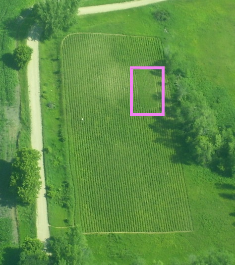
 In 2017 Stuart and Lea relocated and measured 19 individuals of the 381 seedlings originally found. These plants had 1-4 leaves; the longest leaf was 32 cm. It should be interesting to see which individuals are hanging on! In 2017 Stuart and Lea relocated and measured 19 individuals of the 381 seedlings originally found. These plants had 1-4 leaves; the longest leaf was 32 cm. It should be interesting to see which individuals are hanging on!
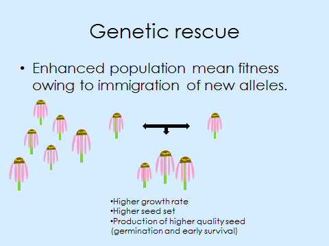
Caroline Ridley established this experiment to compare fitness (recruitment and survival) of seeds originating from individuals with parents from three different backgrounds: 1. both from a large remnant population, 2. both from a small remnant population (not rescued), and 3. one from a large population and one from a small population (genetically rescued). Caroline sowed achenes in an experimental plot at Hegg Lake WMA and marked seedlings with colored toothpicks in May 2009.
Start year: 2008
Site: exPt 4 at Hegg Lake WMA
Overlaps with: crossing experiments qGen1, qGen2, qGen3 & recruitment experiment; INB1
You can find more information about Ridley’s next generation rescue and links to previous flog posts regarding this experiment at the background page for this experiment.
This summer, we measured open-pollinated hybrid Echinacea plants in experimental plot 9 at Hegg Lake. The table below shows the number of plants found alive during each search since the experiment started in 2014. Of the surviving plants in 2017, 90% had fewer than 3 leaves, the mean length of the longest basal leaf was 25 cm, and only six plants had more than one basal rosette. This year we searched for plants once then rechecked every position where we didn’t find a plant during our first search. No plants flowered this year.
| Year / Event |
Number Alive |
% Original remaining |
% Of previous year |
| Planting (2014) |
746 |
100 |
|
| 2014 |
638 |
85.5 |
85.5 |
| 2015 |
521 |
69.8 |
81.7 |
| 2016 |
493 |
66.1 |
94.6 |
| 2017 |
401 |
53.8 |
81.3 |
This experiment comparing the fitness of Echinacea hybrids with pure-bred E. angustifolia and E. pallida will give insight into the possible consequences of non-native E. pallida being planted in restorations in Minnesota, where E. angustifolia is the only native Echinacea.
Measuring at Hegg Lake Start year: 2014
Location: Hegg Lake Wildlife Management Area — experimental plot 9
Overlapping experiments: Echinacea hybrids — experimental plot 6, Echinacea hybrids — experimental plot 7
Data collected: Rosette number, length of all leaves, herbivory for each plant collected electronically and exported to CGData. Recheck information for plants not found was also collected electronically and stored in CGData.
You can find out more information about experimental plot 9 and flog posts mentioning the experiment on the background page for the experiment.
|
|




 In 2017 Stuart and Lea relocated and measured 19 individuals of the 381 seedlings originally found. These plants had 1-4 leaves; the longest leaf was 32 cm. It should be interesting to see which individuals are hanging on!