|
|
2:00 pm winds WSW
1 ew left/row [?]
Tape ends at 18.8m on the N side and 18.85 on the S side.
Plant at 0, 0.33, 0.67 m.
Flags at even meters (ending at 18.04).
Two Oenothera 1-yr olds at N edge 10.45m and 11.00 m.
Weeded Poa, Brome, Carduus, Cirsium, Euphorbia (before planting).
Zer[o] at westernmost grass.
[entered from notes in 2012; see plantOenotheraNov2011.pdf]
In a paper just published in PLoS ONE, Echinacea Project researchers show how habitat fragmentation may make plants more susceptible to aphid attacks. Aphid abundance early in the season is higher on inbred and outcrossed Echinacea angustifolia plants compared to regular plants. Elemental stoichiometry plays a role in this plant-herbivore interaction, but other genetically-based plant traits must also attract or encourage aphids.
Ridley CE, Hangelbroek HH, Wagenius S, Stanton-Geddes J, Shaw RG, 2011 The effect of plant inbreeding and stoichiometry on interactions with herbivores in nature: Echinacea angustifolia and its specialist aphid. PLoS ONE 6(9): e24762. Available online at http://dx.plos.org/10.1371/journal.pone.0024762.
Flowering of Echinacea angustifolia in almost all prairie remnants was down this year. Overall, approximately half as many plants flowered this year as last. Two areas distinctly bucked the trend: flowering was high at Hegg Lake WMA, which was burned this spring, and at our main experimental plot, which was burned this spring. Burning really encourages flowering!
We finished our first round of mapping all flowering plants in nearby remnants and a summary of the raw dataset is shown below. Each line lists the name of a site and the count of demo records and survey records at the site–also the difference in counts. We call our visits to remnants to find and refind plants “demography,” or demo for short. We call mapping the plants surveying because we used to use a survey station. Now we use a survey-grade RTK GPS (a Topcon GRS-1).
      site demo surv diff
1        x    1    0    1
2       aa  131  103   28
3      alf   79   52   27
4      btg    8    3    5
5       cg   20    5   15
6      dog    4    2    2
7     eelr   60   44   16
8      eri  153  122   31
9      eth    9    3    6
10      gc    7    1    6
11      kj   61   44   17
12    krus   69   21   48
13      lc    0    0    0
14     lce   58   45   13
15     lcw   48   31   17
16      lf    0    0    0
17     lfe   77  117  -40
18     lfw   65    0   65
19     lih    2    0    2
20    mapp    5    3    2
21    ness    7    3    4
22     ngc   28   12   16
23   nnwlf   20    7   13
24    nrrx   42   27   15
25    nwlf   27   10   17
26    on27   71   85  -14
27      ri  241  210   31
28     rlr    0    0    0
29    rndt   10    2    8
30     rrx   70   51   19
31   rrxdc    4    0    4
32     sap   80   38   42
33     sgc   10    4    6
34    sign    0    0    0
35     spp  126   78   48
36      th   19   12    7
37   tower   10    3    7
38 unknown    8    0    8
39     waa   10    6    4
40    wood   33   21   12
41     yoh   23    8   15
Notice that most sites have more demo records than survey records. This is because each data recorder enters an empty record at the beginning and end of demoing a site. Also, in certain circumstances we do demo on non-flowering plants.
Something strange is going on with the on27 site. I think someone may have entered the incorrect site name when doing demo. Also, lf looks strange, but is easily explained: lf is divided into two hills (lfe and lfw). We distinguished the two when doing demo, but not when surveying. Our next field activity is to verify the demo and survey dataset and make sure everything makes sense. Being people, we sometimes make mistakes in data entry. Because we know we make mistakes, we generate two separate datasets of flowering records (demo and surv) and compare them. When records don’t match, we go back and check.
We assess survival and reproduction of Echinacea plants in remnants to understand the population dynamics of these remnant populations. We want to know if the populations are growing, holding their own, or shrinking. To figure this out will take a few years because plants live a long time. Estimating a population’s growth trajectory based on just a couple of years of flowering records probably won’t be that informative.
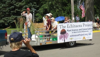
We made an Echinacea Project float and participated in the annual Harvest Festival Parade in Hoffman, MN. It was great fun!

This is how our float was announced… “Native prairies are very rare in Minnesota, but there are several prairie remnants in the Hoffman area. Every summer a team of scientists from around the country comes to study the biology, conservation, and restoration of prairie plants and insects. They are based in the Hoffman – Kensington area. If you see members of The Echinacea Project working on a hillside or in a ditch, ask them what they are doing!”

Team Echinacea is busy in two states! The Minnesota crew is working in the field and the dedicated crew of volunteers at Chicago Botanic Garden in Illinois is working in the lab. This panoramic image of the lab, taken by Bob Mueller, shows volunteers counting Echinacea seeds and taking random samples for weighing. Click & drag the image to see all 360 degrees!
12 August 2011 The Echinacea Project established a new website at echinaceaProject.org.
A quick list of flowering plants I noticed while assessing phenology in Jennifer’s experimental plot at Hegg Lake WMA on 10 July. I list only plants observed in the plot. Asclepias speciosa is flowering just outside the SE corner of the plot.
F = flowering
X = done flowering/in fruit
N = not yet
Heliopsis helianthoides F
Amorpha canescens N
Coreopsis palmata F
Rosa arkansana F
Anemone cylindrica X
Silene F
Asclepias syriaca F
Amphicarpea bracteata F
Morning glory sp F
Apocyanum F
Tragopogon F
Cirsium arvense F
Lathyrus venosus XF (almost all done flowering)
Galium boreale F
Psoralea argophylla F
Medicago sativa F
Linum sulcatum F
Carduus acanthoides F
Senecio X
Liatris N
Achillea F
Zizea X
Red field clover F
Yellow fl lactucid F
Potentiall arguta F
Desmodium F
Physalis F
Dichanthelium leibergii XF
No Phlox pilosa in the plot!
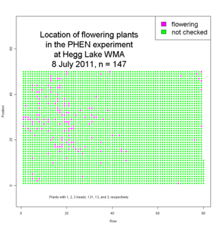
We found 147 flowering plants in Jennifer’s Phenology Experiment during a thorough, but not exhaustive, search on Friday. Most of these plants have buds only and will start shedding pollen later. I posted a map of locations of all plants to flower this year.
 Click on thumbnail to see a larger map. Click on thumbnail to see a larger map.
Jennifer planted this experiment to investigate heritability of flowering timing (phenology) in spring 2006.
Last year eight plants flowered and about 2700 plants were alive. Read about measuring last year.
Assuming that almost all of those plants are still alive and that we didn’t find all the flowering plants, then about 6% of surviving plants will flower this year (>147/2700).
For kicks, I made maps of the paths of data enterers. We usually worked in pairs and used one person’s PDA to enter data. Here are the paths…
Josh D’s visor, Amber E’s, Nicholas G’s visor, Gretel K’s visor, Lee R’s visor, Callin S’s, Stuart W’s visor, Maria W’s visor, Amber Z’s visor. For the record Katherine M’s visor had only one record and we didn’t use Karen T’s visor.
24 May 2011 Megan Kate Gallagher defended her Master’s Thesis in Plant Biology and Conservation at Northwestern University. Congratulations! For her thesis project, Kate demonstrated how performance of three dominant prairie grasses in restorations depended on seed source. This fall Kate will start the PhD program in Ecology and Evolutionary Biology at the University of California–Irvine working with Diane Campbell.
We designed an experiment to assess how fire affects the growth of plants. This spring we will plant about 2500 seedlings in 2500 randomly assigned locations on a 1m x 1m grid. We aim to keep track of the identity of all individuals and plant them quickly and efficiently. Here are five datasheets that will help: pathsToPlant.pdf, plantingDataSheet.csv, plugRowsPerPath.pdf, trayInfoByPseg.pdf, trayInfoByRow.pdf
|
|