After 5 months of preparation, we officially applied the first experimental treatments for our NSF proposal to study prescribed fire effects on prairie plant reproduction and population dynamics.
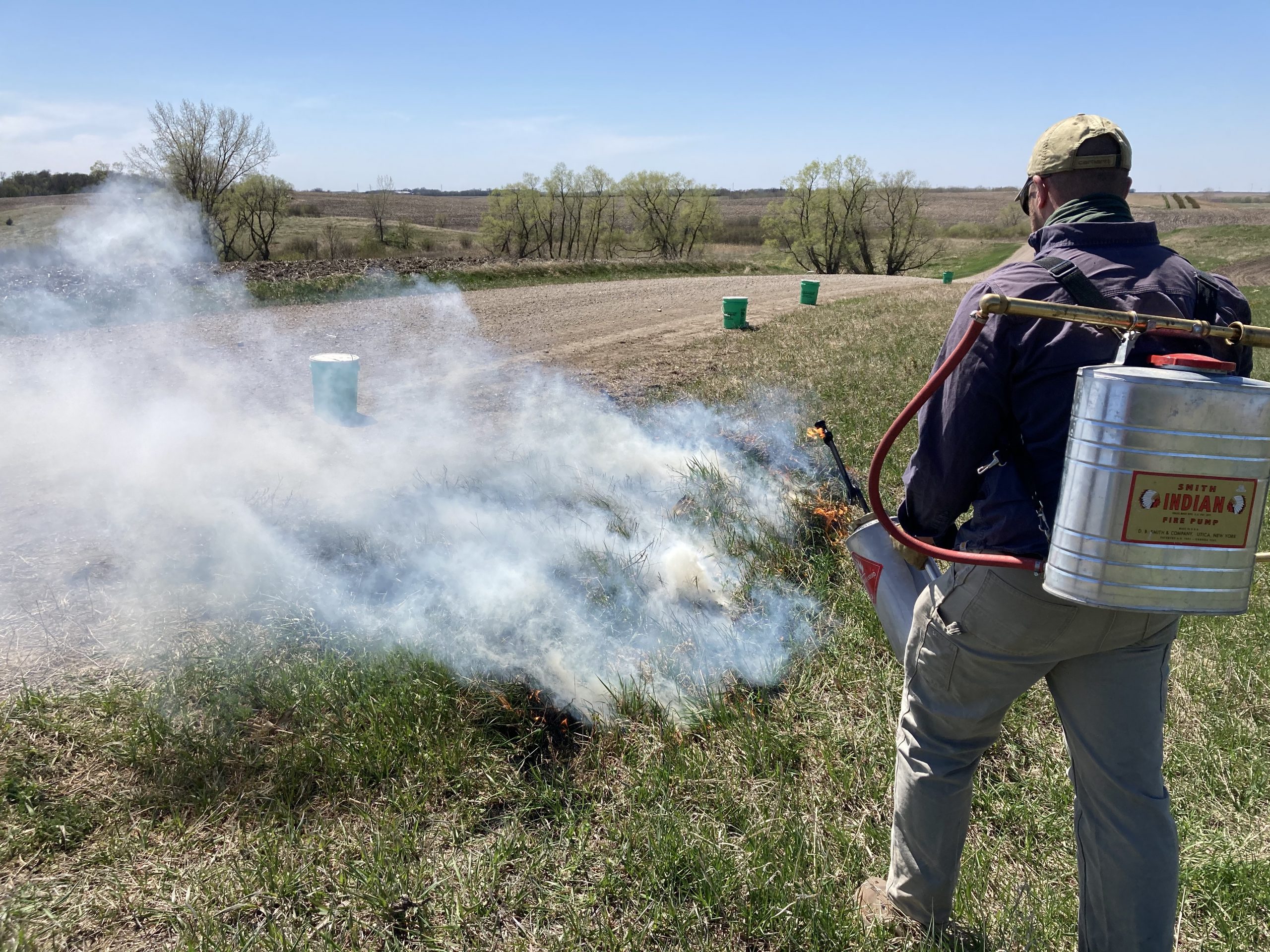
Weather conditions Tuesday afternoon were favorable for burning but wind forecasts were at the upper end of our burn prescription. Given our success burning p8 in similar conditions just a week earlier, we decided to proceed cautiously by starting with a prescribed burn on the north side of east riley. Here light and discontinuous fuel (mostly brome), a gravel road for a firebreak on the south side, and agricultural fields downwind mitigated our concerns about gusty winds. Earlier in the day, Mia mowed fire breaks along the east and west end of the burn unit. We ate lunch, loaded up our equipment, and drove down to east riley. Along the way, the crew got a great look at a western kingbird perched along Sandy Hill Road.
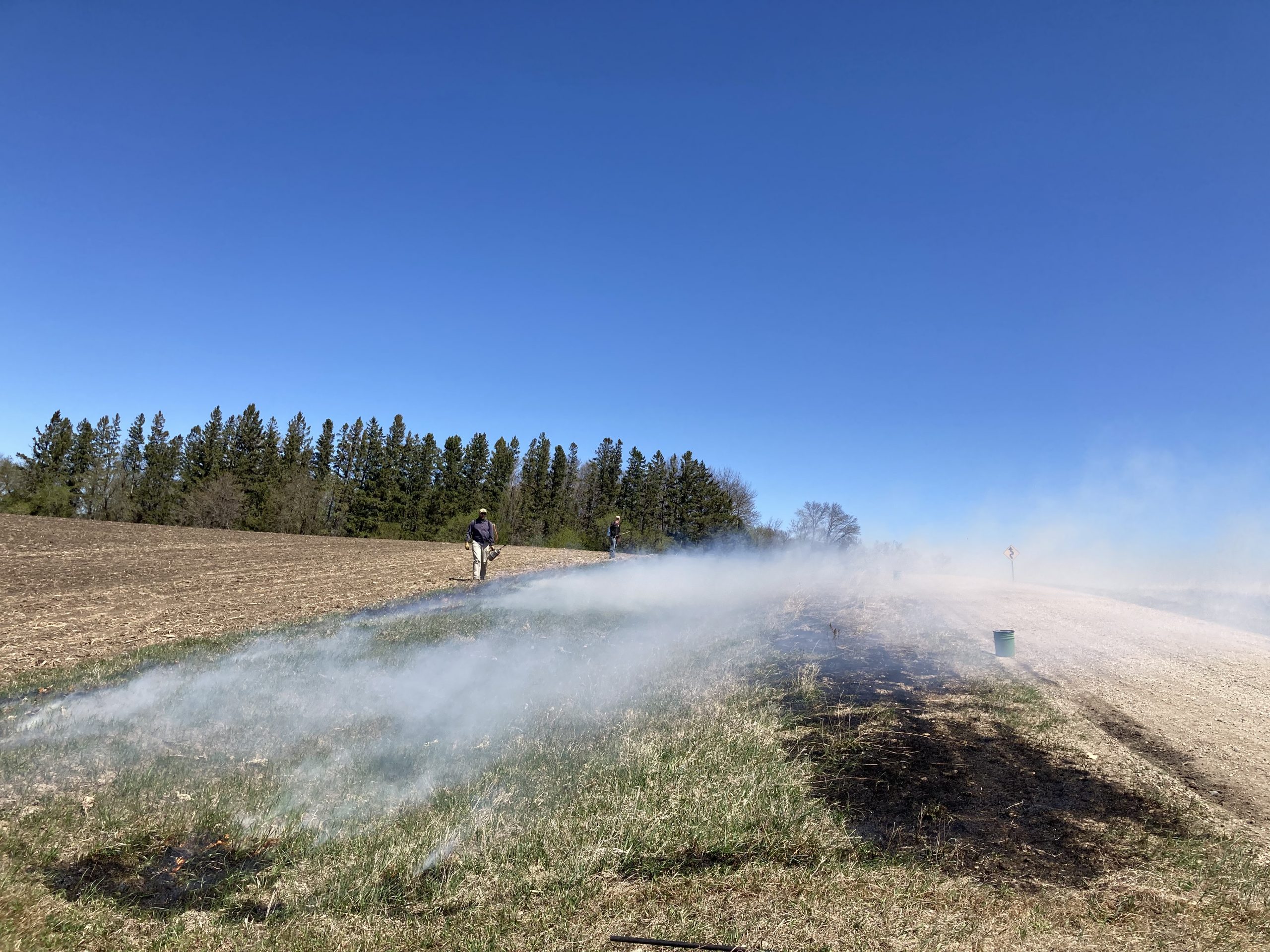
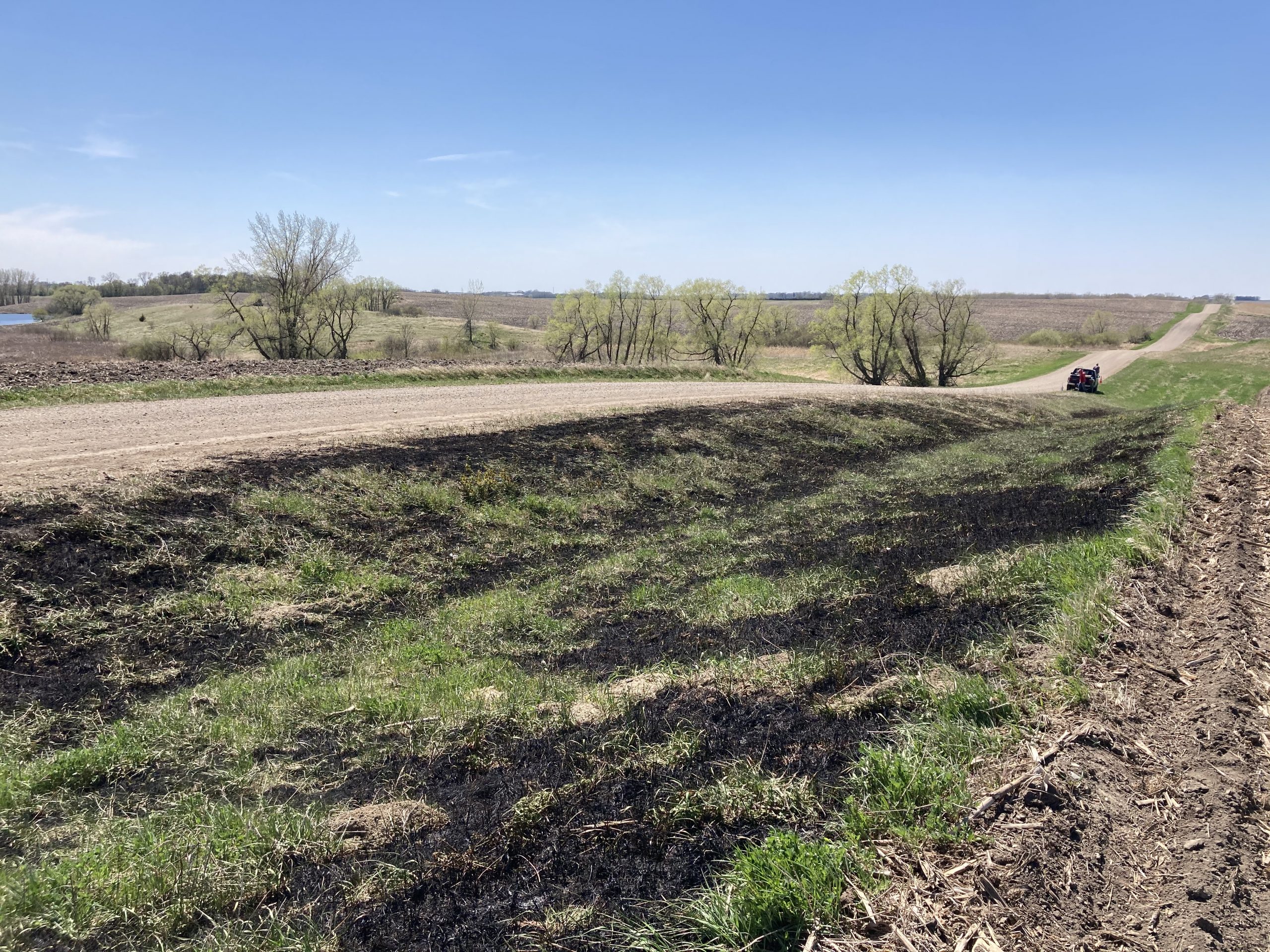
Once at the site, we reviewed the burn plan and staged equipment. We ignited a test fire in the southeast corner of the burn unit. Despite a slow start to the test fire and stiff NW winds that kept extinguishing the drip torch, the backing fire burned well through brome and scattered warm season grasses. With scattered poison ivy in the eastern third of east riley, we were cautious to stay upwind of smoke by lighting small strips perpendicular to the wind. Once sufficient black (burned area downwind) had been established, we proceeded to ignite the southern edge of the unit along Mellow Ln and wrap around the western end of the unit to ignite a head fire along the northern edge of the burn unit.
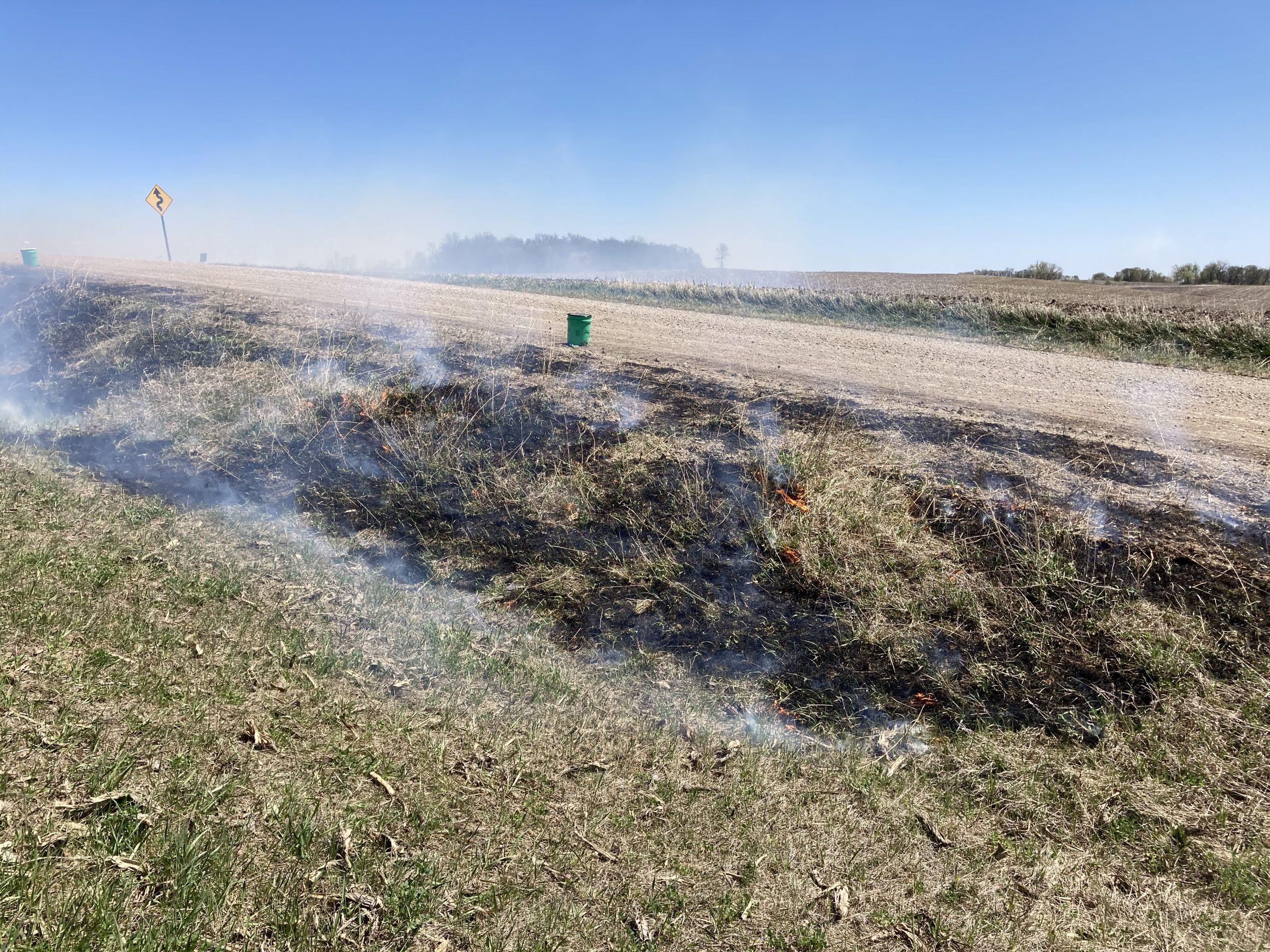
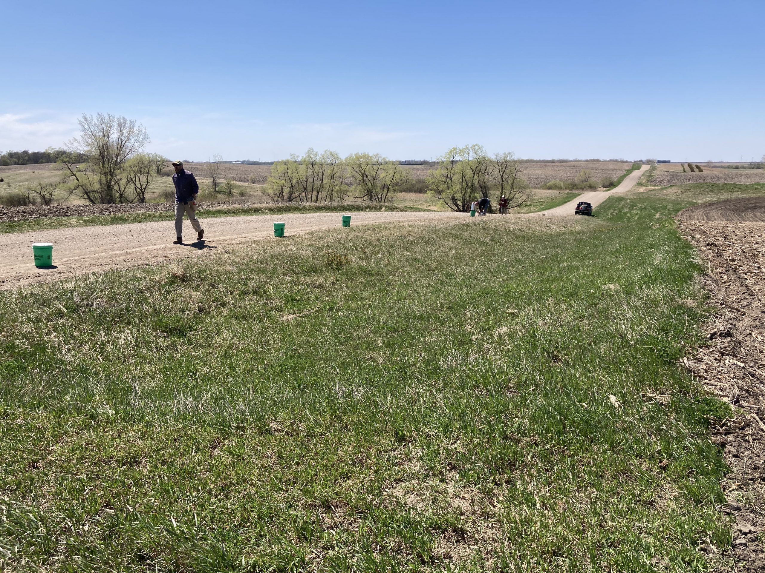
While somewhat patchy, we considered the burn a success. The fire behaved predictably and we felt comfortable that we could continue burning other units with more fuel. After the burn, Stuart shared the observation that the fire did not carry well in areas where fuel was covered by a film of silt/gravel. We packed up and drove a short distance into Grant County for our next set of burn units…
Temperature – 52 F Relative humidity – 34% Wind speed (max gusts) – 13 (22) mph wind direction – NNW Ignition time – 2:22 PM End time – 2:58 PM Burn crew: Jared, Stuart, Gretel, Mia
Before and after comparison looking west along Mellow Ln.
This summer Team Echinacea did demo and surv in 42 prairie remnants and other sites with Echinacea angustifolia populations. Demo involved measuring traits of individual plants: flowering status, number of flowering heads, and near neighbors. This summer we took 5119 demo records on our handheld data collectors (visors). Surv involved tagging individual plants and recording their location with our super-precise GPS (Darwin). This summer we shot 1494 points for surv. For ‘total demo’, we navigated to adult Echinacea plants that have been previously visited and took demo to generate detailed, long-term records of individual fitness in these fragmented Echinacea populations. At smaller sites we collected data on all adult plants and at larger sites we visited a subset of the adult plants. The demo and survey datasets are in the process of being combined with previous years’ records of flowering plants in “demap,” the spatial dataset of remnant reproductive fitness that the Echinacea Project maintains.
Start year: 1995
Location: Remnant prairie populations of the purple coneflower, Echinacea angustifolia, in Douglas County, MN. Sites are located between roadsides and fields, in railroad margins, on private land, and in protected natural areas.
Total demo: Bill Thom’s Gate, Common Garden, Dog, East of Town Hall, Golf Course, Hegg Lake, Martinson’s Approach, Nessman, North of Golf Course, REL, RHE, RHP, RHS, RHX, RKE, RKW, Randt, Railroad Crossing Douglas County, South of Golf Course, Sign, Town Hall, Tower, Transplant Plot, West of Aanenson, Woody’s, Yellow Orchid Hill
Annual sample: Aanenson, Around Landfill, East Elk Lake Road, East Riley, KJ’s, Krusemarks, Loeffler’s Corner, Landfill, North of Railroad Crossing, Northwest of Landfill and North of Northwest of Landfill (lumped), On 27, Riley, Railroad Crossing, Steven’s Approach, Staffanson Prairie
Data: Dropbox/geospatialDataBackup2020 contains the experiment’s GPS files and the aiisummer2020 repo contains its demo records. The most recent copies of allDemoDemo.RData and allSurv.RData are accessed at Dropbox/demapSupplements/demapInputFiles.
Products: Amy Dykstra’s dissertation included matrix projection modeling using demographic data. The “demap” project merges phenological, spatial and demographic data for remnant plants.
For more information on demographic census in the remnants, visit the experiment’s background page, or explore flog entries that mention the experiment.
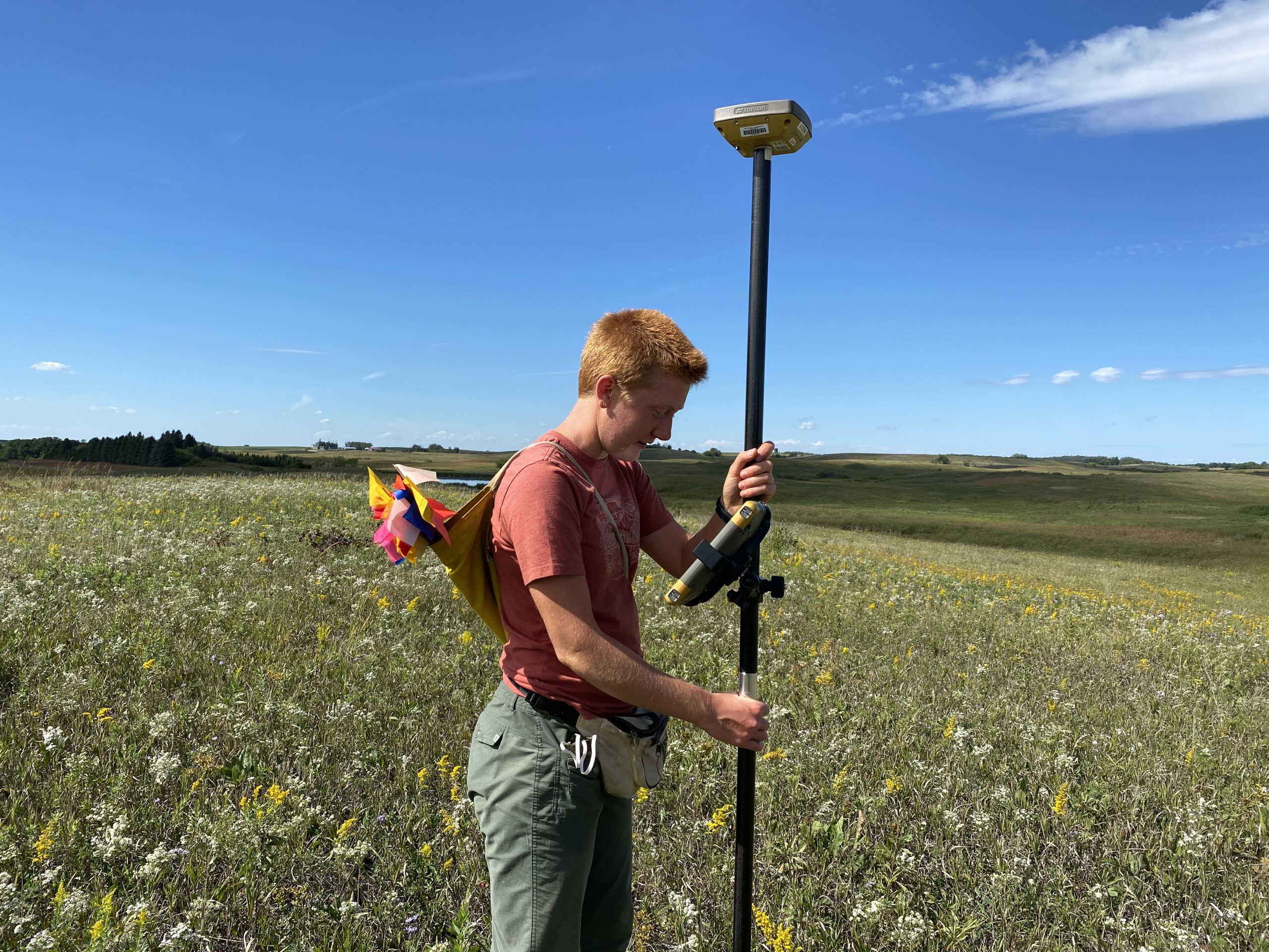
Emma using Darwin, our survey-grade GPS, in late August near Hegg Lake
Poor weather conditions delayed demo this year but did not
dampen our spirits! In 2019 Team Echinacea added 4031 visor records to demo and
1431 GPS points to surv. The largest effort this summer occurred at Aanenson
where eight team members took demo records on over 200 flowering plants. We
found flowering plants at Northwest of Landfill with tags from 1995 in situ, meaning the plants were at
least several years older than most of the team. We also found non-angustifolia
Echinacea invading prairie remnants Dog and Yellow Orchid Hill.
The team does demo at everyone’s favorite site: East Riley! Also known as Whose Loc Is It Anyway? Where the status is “Can’t find” and the GPS points don’t matter.
This year we performed demo and surv at 32 prairie remnants
and 10 additional sites with angustifolia populations. For our smaller sites we
visit every mature plant (ones which have flowered before.) At the larger sites
we measure a subsample of the mature population. At every site we also perform
flowering demo, where we visit plants which flowered for the first time or were
not included in the subsample. We record the status of each plant we visit, its
neighbors and the number of heads it produced. All flowering plants are tagged
and shot in surv, and in the coming months we will use demap to reconcile the
2019 demo and surv records with each other as well as those from previous years
to construct our spatial dataset of reproductive fitness in the tallgrass
prairies of our study area.
Total Demo Bill Thom’s Gate, Common Garden, Dog, East of Town Hall, Golf Course, Hegg Lake, Martinson’s Approach, Nessman, North of Golf Course, REL, RHE, RHP, RHS, RHX, RKE, RKW, Randt, Railroad Crossing Douglas County, South of Golf Course, Sign, Town Hall, Tower, Transplant Plot, West of Aanenson, Woody’s, Yellow Orchid Hill
Annual Sample Aanenson, Around Landfill, East Elk Lake Road, East Riley, KJ’s, Krusmark’s , Loeffler’s Corner, Landfill, North of Railroad Crossing, Norwest of Landfill and North of Northwest of Landfill (lumped,) On 27, Riley, Railroad Crossing, Steven’s Approach, Staffanson Prairie
In addition to the annual collection of data, this year Erin
began developing a study to investigate whether flowering return interval and
isolation by distance are correlated in Echinacea.
Start year: 1995
Location: Unbroken (never tilled) remnant prairies in Douglas County, MN, located along roadsides, nature preserves, railroad right-of-ways and privately-owned land.
Data: Access the most recent copies of allDemoDemo.RData and allSurv.RData at ~Dropbox\demapSupplements\demapInputFiles. Demap accepts these files and the demap team will clean and reconcile them in the demap repository. ~Dropbox\geospatialDataBackup2019 houses the raw GPS jobs while the aiisummer2019 repo houses the raw demo records.
Data related to
the flowering isolation study can be found in the floiso repository (contact
Erin Eichenberger for access) and in the folder ~Dropbox\floweringIsolation2019
Products: Amy Dykstra’s dissertation included matrix projection modeling using demographic data
Project “demap” merges phenological, spatial and demographic data for remnant plants
You can read more about the demographic census in the remnants, as well as links to prior flog entries mentioning the experiment, on the background page for this experiment.
On 21 Dec 2019 demap was updated to accept 2019 demography and survey records. In 2019 we took 4031 visor records in demo and 1413 GPS points in surv. The updated infiles are located in ~Dropbox\demapSupplements\demapInputFiles. Demo and surv have not yet been reconciled.
2019 should be the last year we use a GRS-1 machine, as Chekov is set to be decommissioned this spring. Thanks, Chekov! He was truly a key player while Darwin was in surgery for his busted receiver.
As always, demo was a huge job this year. This season we added 3868 demo records and about 1539 survey records to our database. After over 20 years of this method, we are starting to get a very good idea of the demography of Echinacea in Solem Township.
So how do we do demo? When we find a new flowering Echinacea plant, we give it a tag and get its location with a survey-grade GPS (better than 6 cm precision). Then, we can revisit this plant for years to come and monitor its survival and reproduction. We’re monitoring over 10,000 plants as of 2018. With this many records, organizing demap in the future is going to be a big task!
We made some small adjustments to how we do total demo and flowering demo (we do flowering demo in every remnant now). Now, in our big plots, we only do a sample of the plants instead of total demo. Check out the updated table below (remember we did flowering demo everywhere). We still managed to shoot thousands of points, take even more demography records, and, as always, follow the colored flags!
Total Demo
BTG, Common Garden, DOG, East of Town Hall, KJs, Krusemark, Landfill West, Loeffler Corner East, Near Town Hall, Nessman, NNWLF, NRRX, recruit he, recruit hp, recruit hs, recruit el, recruit hw, recruit ke, recruit kw, RRX, RRXDC, South of Golf Course, Steven’s Approach, transplant plot, Tower, Town Hall, West of Aanenson, Woody’s
Sample Demo
Aanenson, Around LF, East Riley, Hegg Lake, Elk Lake Road East, Golf Course, Landfill, Loeffler Corner, North of Golf Course, NWLF, On 27, Riley, Staffanson, Yellow Orchid Hill
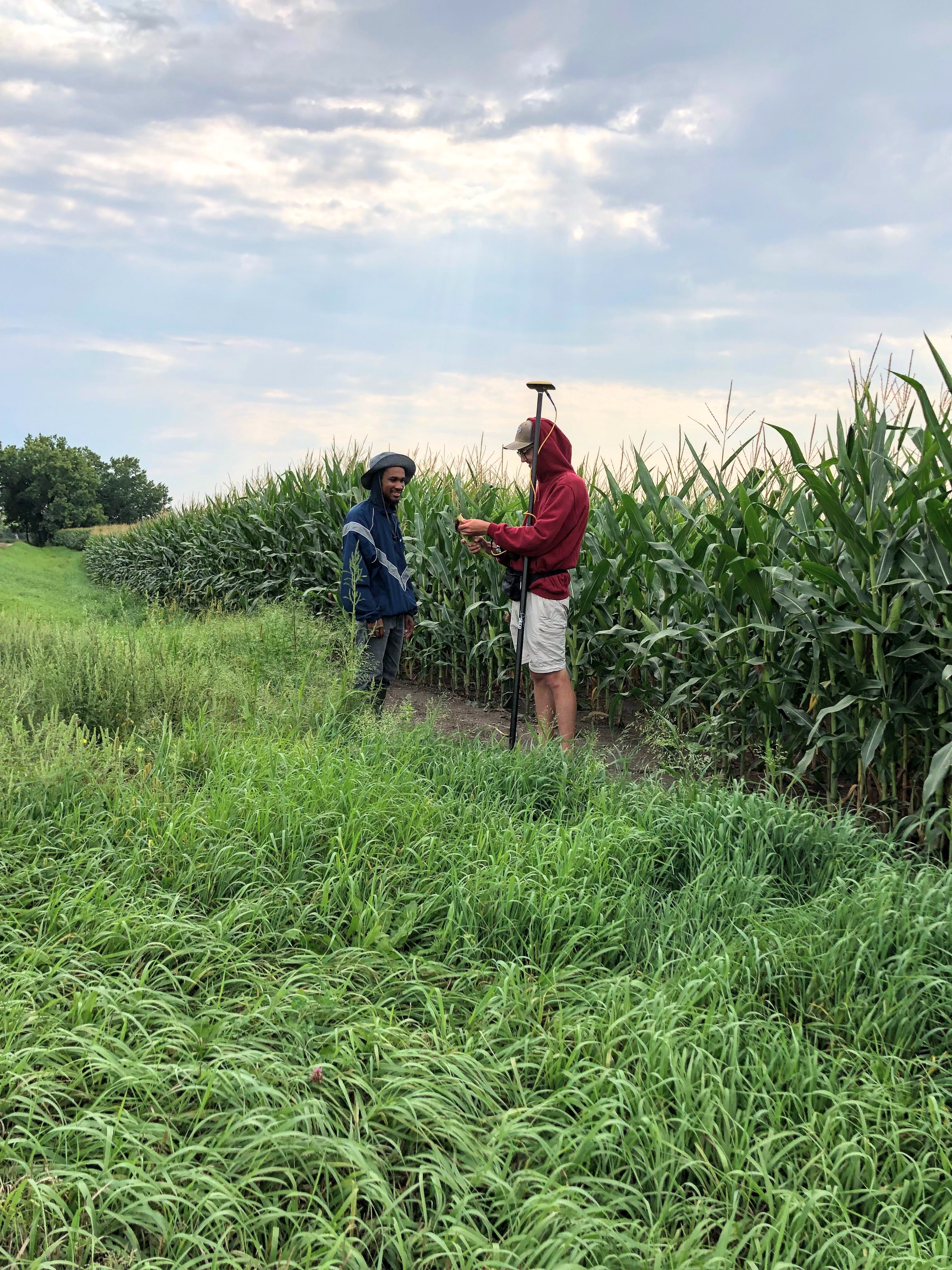
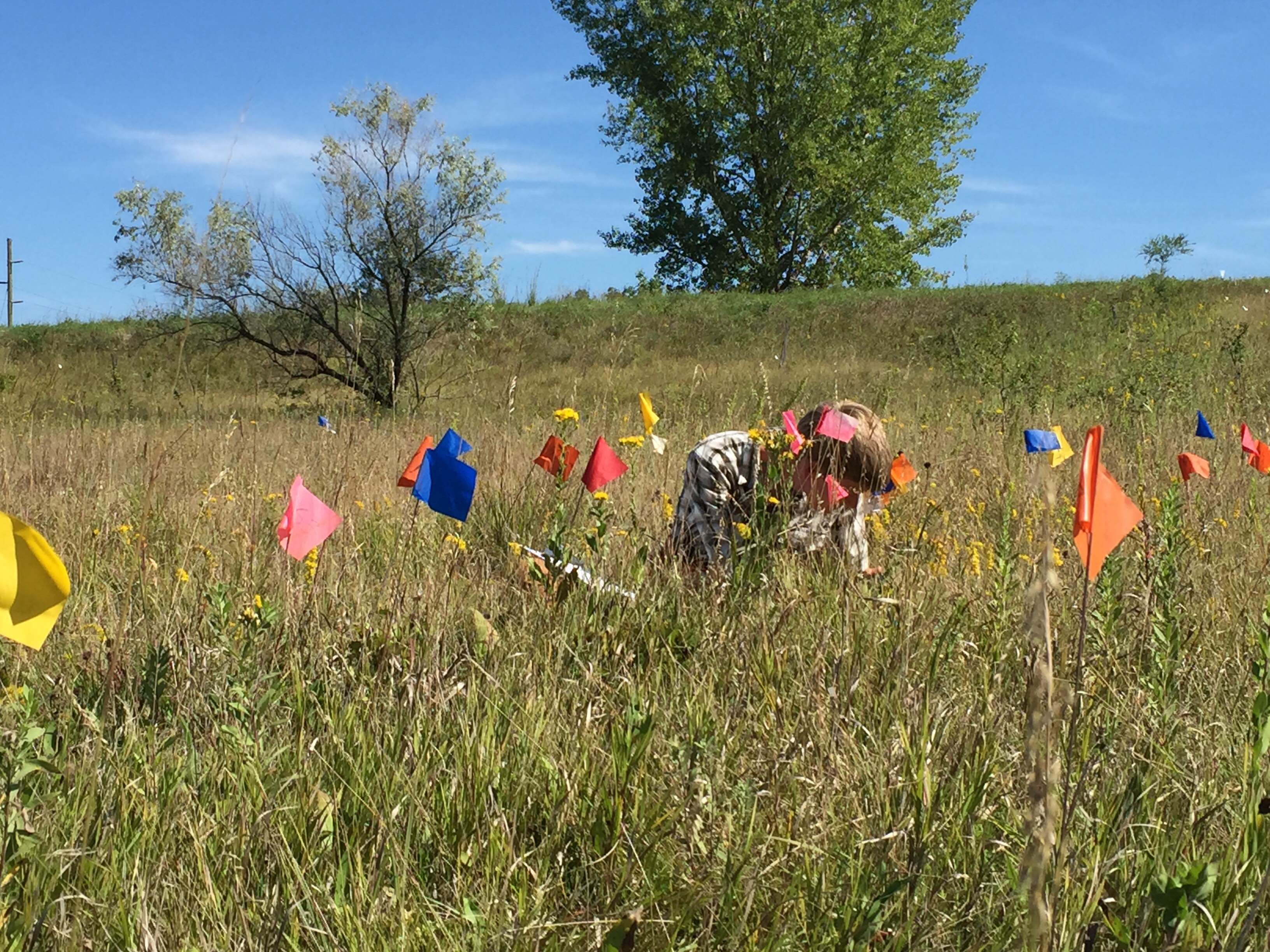
Evan and Will doing demo by the corn. While you might not be able to see the echinacea, we promise, it’s under there!
Year started: 1996
Location: Roadsides, railroad rights of way, and nature preserves in and near Solem Township, Minnesota.
Data collected: demo records include Flowering status, number of rosettes, number of heads, neighbors within a 12 cm radius of plants found. These are all taken with PDAs that sync with an MS Access database. They are all transferred to the demap R repository in bitbucket with git version control.
GPS points shot: Points for each flowering plant this year shot mostly in SURV records, stored in surv.csv. Each location should be either associated with a loc from prior years or a point shot this year.
Products:
Amy Dykstra’s dissertation included matrix projection modeling using demographic data
Project “demap” merges phenological, spatial and demographic data for remnant plants
You can find out more about the demographic census in the remnants and links to previous posts regarding it on the background page for this experiment.
We had a big year for censusing plants in natural remnant populations. In 2017 we did both total demo, visiting all plants, and flowering demo, visiting just plants that flowered this year. Check out the chart below to see what we focused on at each site:
Total Demo
Aanenson, Around LF (partial), Common Garden, East of Town Hall, East Riley, Hegg Lake, Landfill West, Loeffler Corner East, NRRX, recruit he, recruit hp, recruit hs, Riley, RRX, South of Golf Course, Steven’s Approach, transplant plot
Flowering Demo
Around LF, BTG, DOG, Elk Lake Road East, Golf Course, KJs, Krusemark, Landfill East, Liatris Hill, Loeffler Corner West, Near Town Hall, Nessman, NNWLF, North of Golf Course, NWLF, On 27, recruit el, recruit hw, recruit ke, recruit kw, RRXDC, Staffanson East Unit, Staffanson West Unit, Tower, Town Hall, West of Aanenson, Woody’s, Yellow Orchid Hill East, Yellow Orchid Hill West
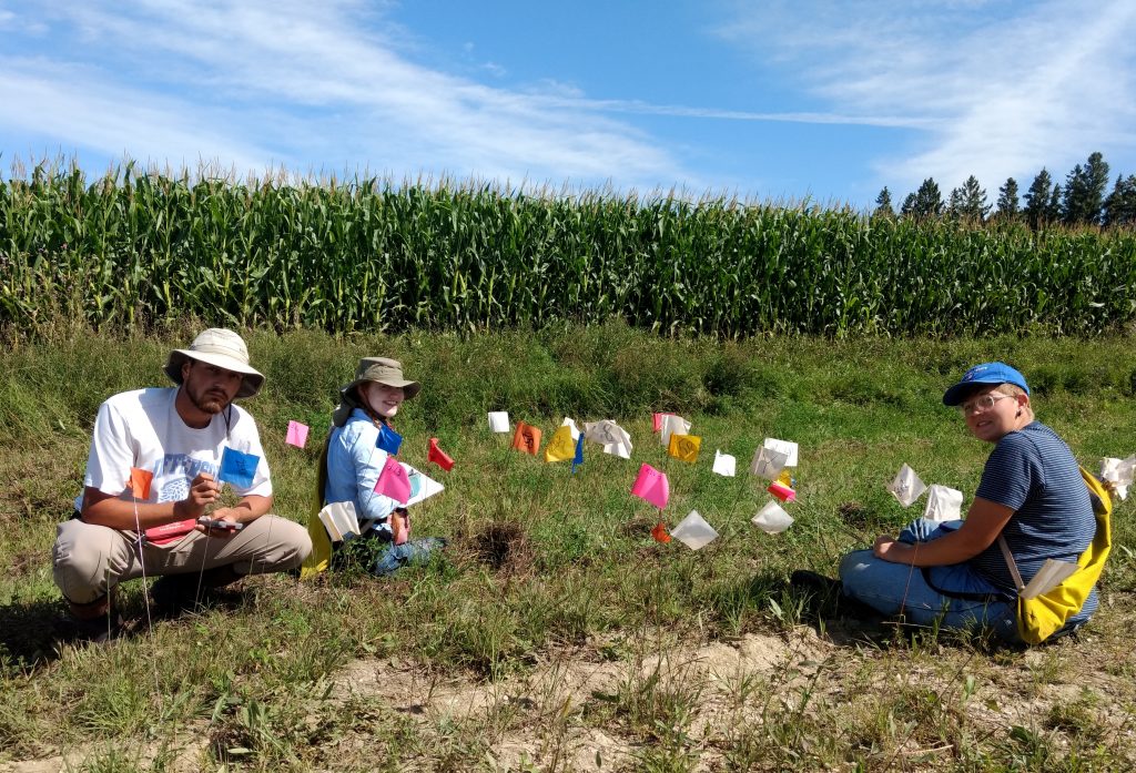
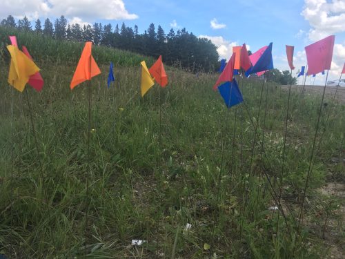
We stake to locations where flowering plants have been found in the past and place a flag there. This is the East Riley roadside remnant, an area with a lot of Echinacea close together and a high chance of getting mowed.
When we find a new flowering Echinacea plant, we give it a tag and get its location with a survey-grade GPS (better than 6 cm precision). Then, we can revisit this plant for years to come and monitor its survival and reproduction.
This season we added 5945 demo records and about 1375 survey records to our database. After over 20 years of this method, we now have a very rich longitudinal dataset of life histories including thousands of plants. REU Will Reed was a huge help organizing demo tasks for Team Echinacea over the summer and helping out with demap (the demographic census database) during the year.
Year started: 1996
Location: Roadsides, railroad rights of way, and nature preserves in and near Solem Township, Minnesota.
Data collected: demo records include Flowering status, number of rosettes, number of heads, neighbors within a 12 cm radius of plants found. These are all taken with PDAs that sync with an MS Access database. They are all transferred to the demap R repository in bitbucket with git version control.
GPS points shot: Points for each flowering plant this year shot mostly in SURV records, stored in surv.csv. Each location should be either associated with a loc from prior years or a point shot this year.
Products:
Amy Dykstra’s dissertation included matrix projection modeling using demographic data
Project “demap” merges phenological, spatial and demographic data for remnant plants
You can find out more about the demographic census in the remnants and links to previous posts regarding it on the background page for this experiment.
We revisited locations in remnants where flowering plants were observed in previous years.
We tag each Echinacea plant we see flowering in our prairie remnants, and record its location using the GPS. This is useful because it allows us to revisit the same plant in future years, checking to see if it is still alive, and if so how large it is and whether or not it is flowering. This has provided us with a very rich longitudinal dataset of life histories, dating back two decades and including thousands of plants. This year, we did total demo, visiting each plant in our database, at several sites including Staffanson, Loeffler’s Corner East, Northwest of Landfill, and East Elk Lake Road. In the interest of time, we only did flowering demo (only visiting plants that flowered this year) at several sites, including Landfill, Around Landfill, and Railroad Crossing. For each plant visited, we recorded its status (e.g., basal, flowering), its number of rosettes, and any neighboring Echinacea within a 12 cm radius. This data can be used to study inter-annual variation in flowering, population dynamics, and response to fire.
Year: 1996
Location: Roadsides, railroad rights of way, and nature preserves in and near Solem Township, Minnesota.
Data collected: Flowering status, number of rosettes, number of heads, neighbors within a 12 cm radius of plants found, stored in demo2016
GPS points shot: Points for each flowering plant this year shot mostly in PHEN records, stored in surv.csv. Some points of flowering plants stored in SURV records, also in surv.csv. Each location should be either associated with a loc from prior years or a point shot this year.
Products:
Amy Dykstra’s dissertation included matrix projection modeling using demographic data
Project “demap” merges phenological, spatial and demographic data for remnant plants
You can find out more about the demographic census in the remnants and links to previous posts regarding it on the background page for this experiment.
This winter we’ve been working on ‘demap’, a project to coordinate 20+ years of demography and spatial data from remnant populations of Echinacea in Solem Township. When we are done we will have a great long-term dataset of over 3000 individuals in 27 remnant populations. We can use that information to answer all kinds of questions about flowering dynamics in natural populations, population growth, and the consequences of disturbances such as habitat fragmentation and fire! In particular, this January we focused our efforts on answering questions about the demographic consequences of fire. Does fire’s stimulation of flowering contribute to increased population growth over the long term? Do reproductive benefits of fire outweigh potential survival costs? We’re not sure, but we hope to find out by analyzing four populations– a large population that had one fire event, a large population that has not been burned in the past 20 years, a small population that burned once, and a small population that has not burned in the past 20 years. We’ll combine our demography data about flowering and survival with other information, such as the seedling recruitment and remnant seed set data, to project population growth.
Will was here to help out with the project in the first two weeks of January. We got a lot done with demap and made meaningful progress on other big questions such as “Is kale overrated?” and “What does overrated mean statistically?”. We also made big strides in terms of professional development by studying business mogul DJ Khaled’s keys to success. Stay tuned for updates!
Sincerely,
Amy
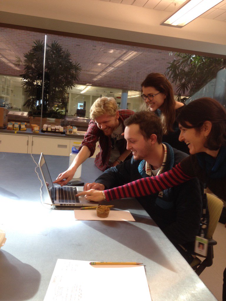
Demap is a team effort! In this shot, we are helping Will find a plant on the computer.
Today was probably the coldest day of fieldwork we have had all summer, a cold front passed through on Wednesday and left us with a cloudy 60 degree day. For those team members who are more accustomed to hotter summers today was a little bit of a shock.
We went out to do total demography at Staffanson Praire Preserve, our goal while doing total demo is to census all of the plants that have flowered sometime in the last 20 years. It’s a big project, at Staffanson alone there are just over one thousand locations to visit. While not all of these locations still have a plant it is awesome to see a tag around a plant that was put there in 1996 or 1997.
Even the flowers are cold!
We made a huge dent in the number of locations at Staffanson, of the 1054 locations we visited 435, nearly half done!
Scott stakes locations while Amy does demography on the plants at each location
Here is a proposal for a fun project. It involves using demography data from this (and prior) years to estimate the growth rates of each of the remnants individually. Actually, that’s basically the whole project. Action items for the next month include: reading technical manuals with specifics on implementing aster models (see the list of project publications if you want to read them for me on your own).
In other Scott-research related news, I will also try modeling fitness of various Hesperostipa spartea crosses in experimental plot 1. Just today I got a list of positions of plants found alive in 2016 — my plan in the near future is to search positions in the plot where plants were found alive in 2011 but weren’t found in 2016 to assess mortality. Keep your eyes open for another action-packed research proposal for this porcupine grass-ey project.