My individual project is working on collecting nectar from Echinacea angustifolia. I was tasked with figuring out what equipment is needed to collect nectar, what time of day is best to collect nectar, and what the procedure is to collect nectar. I have been working in P1 for this nectar collection data. Dr. Roy from St. Catherine University in St. Paul, Minnesota came to help me learn about nectar collection and where exactly to collect the nectar from on the plant head. Next summer, the team hopes to collect pollen and nectar to assess the quantity and quality of food resources pre and post-burn.
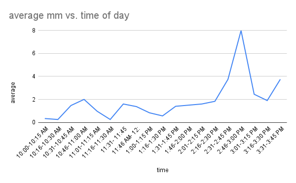
So far, I have learned how to extract the nectar and that around 2:30-3:00 PM has produced the most nectar. Cloudy days are NOT ideal for nectar collection. The one day I collected when it was cloudy I only got 1 mm of nectar the entire morning.
As of today, I have collected 142 mm of nectar. I used different microcaps with different inner and outer diameters, so the volume is not 142 (I need to do some more math to find the volume for each amount depending on their inner diameter, but at least you get an idea of the amount that has been collected).
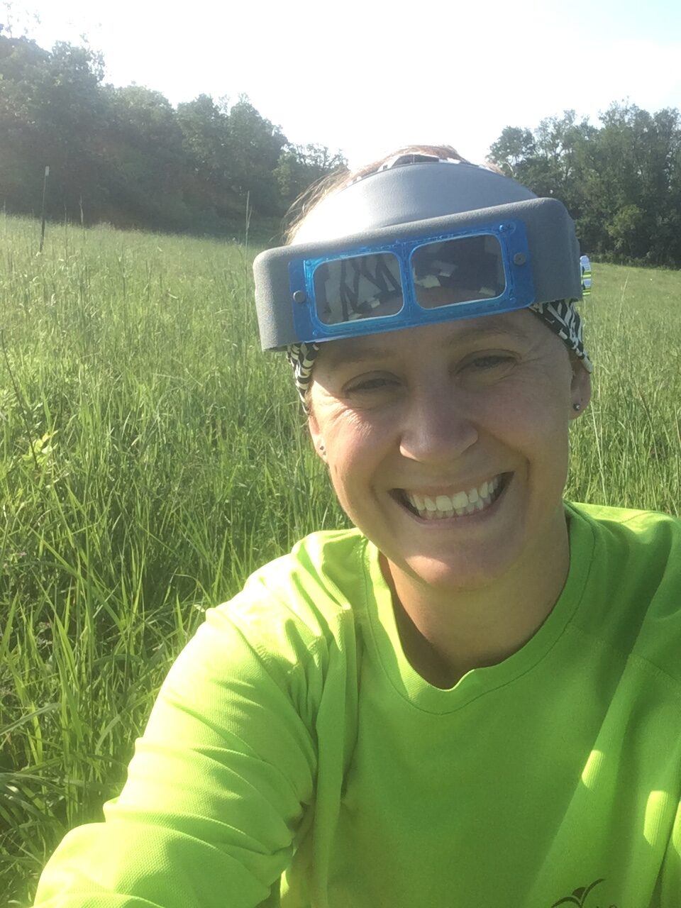
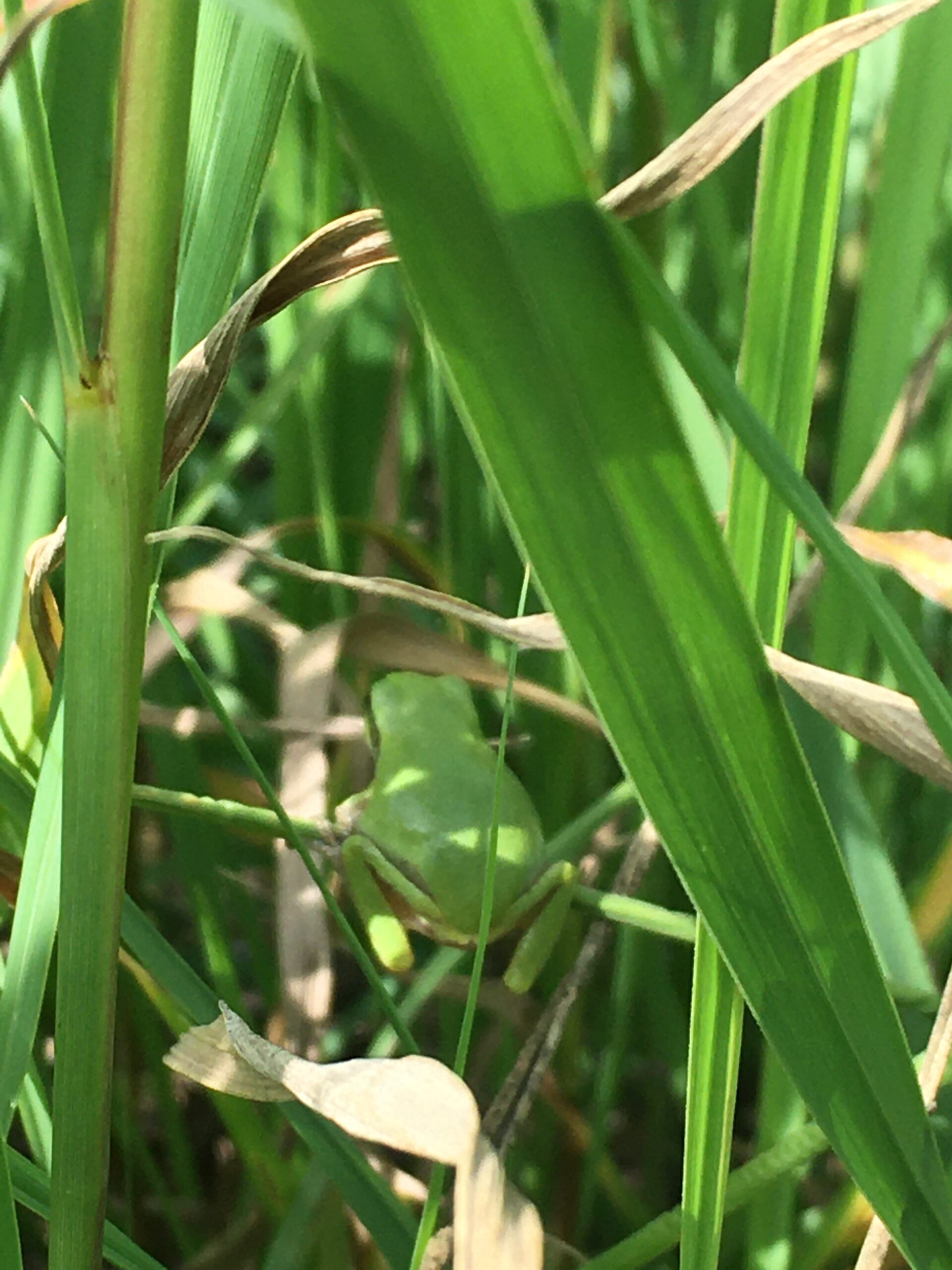
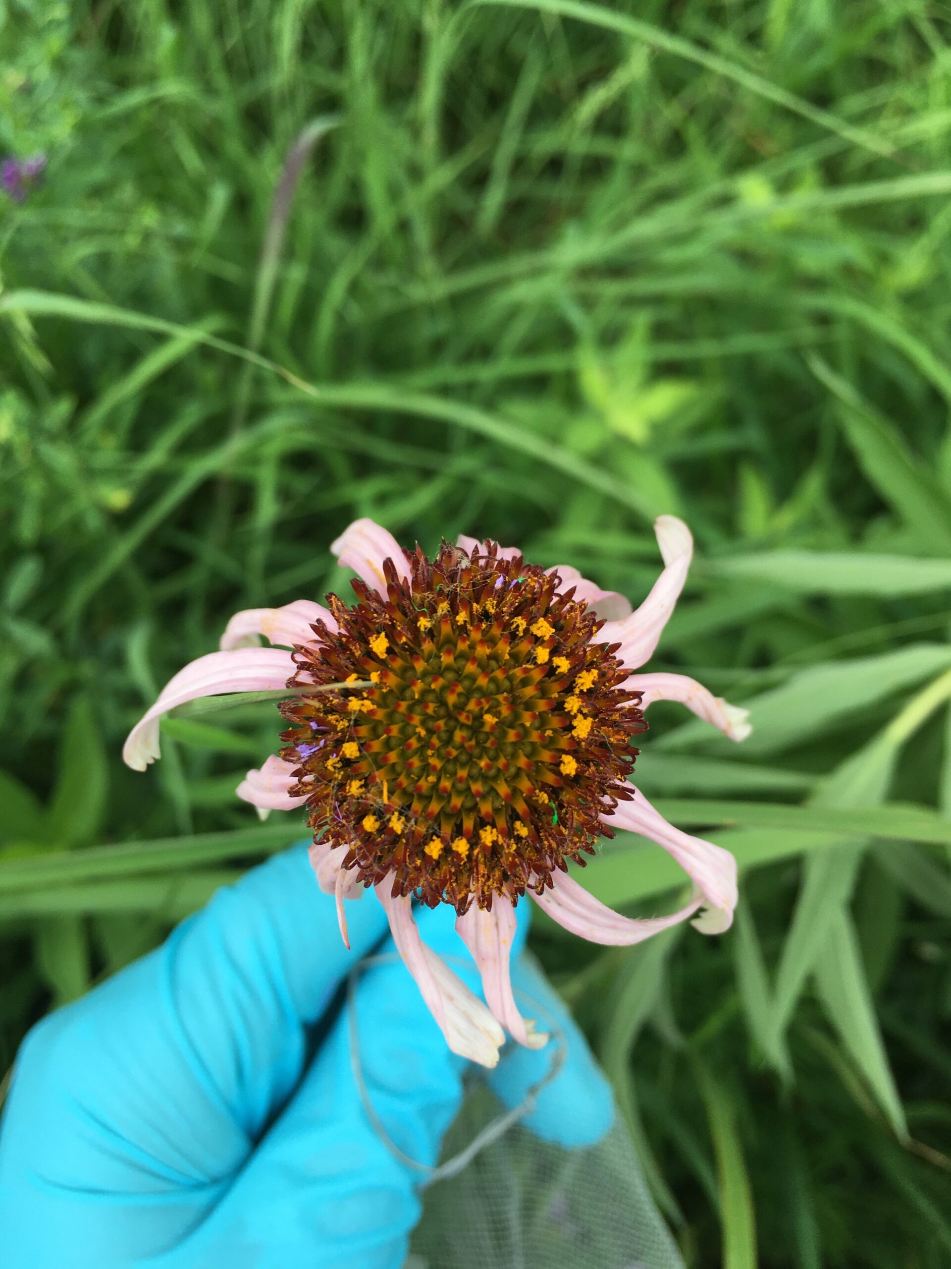
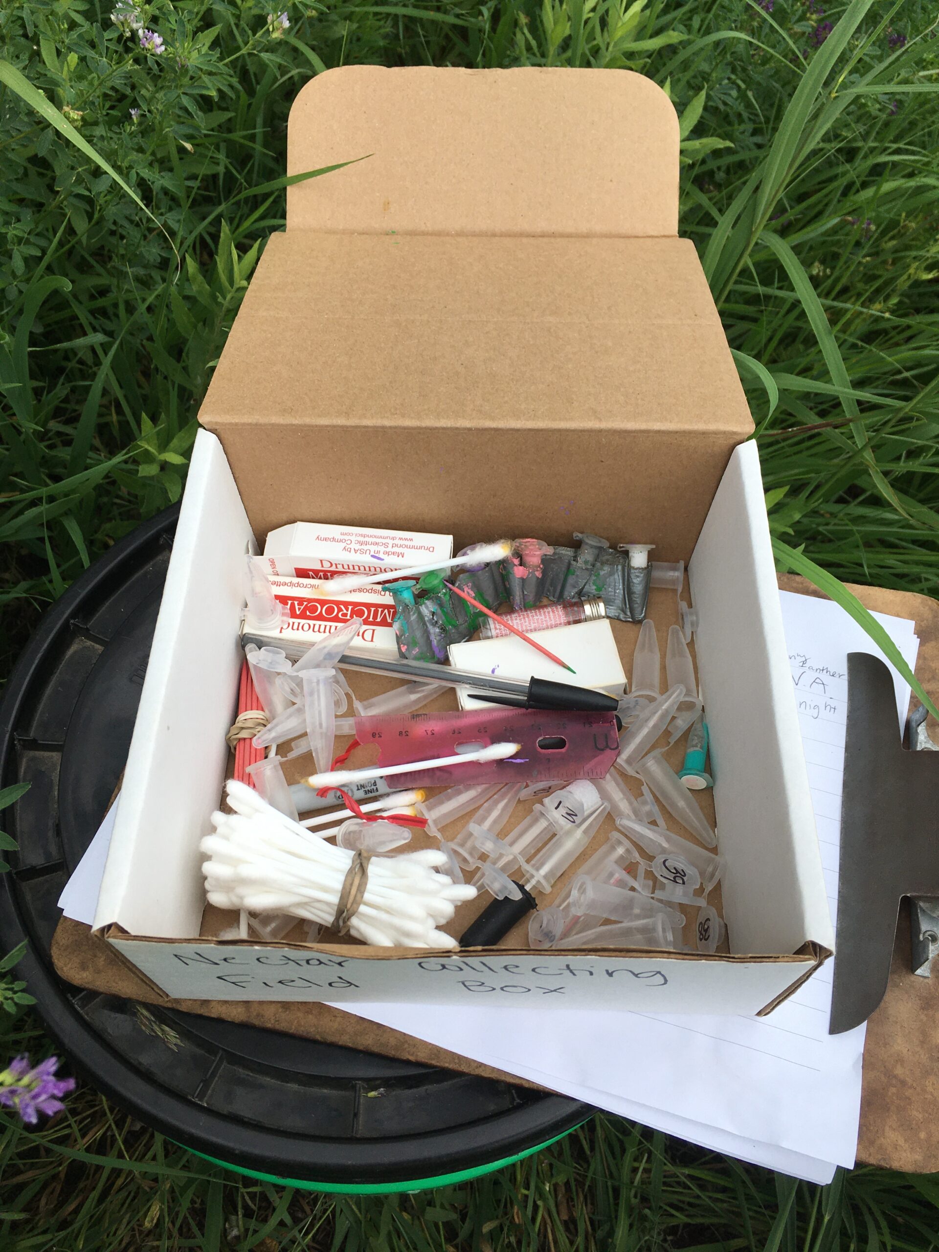
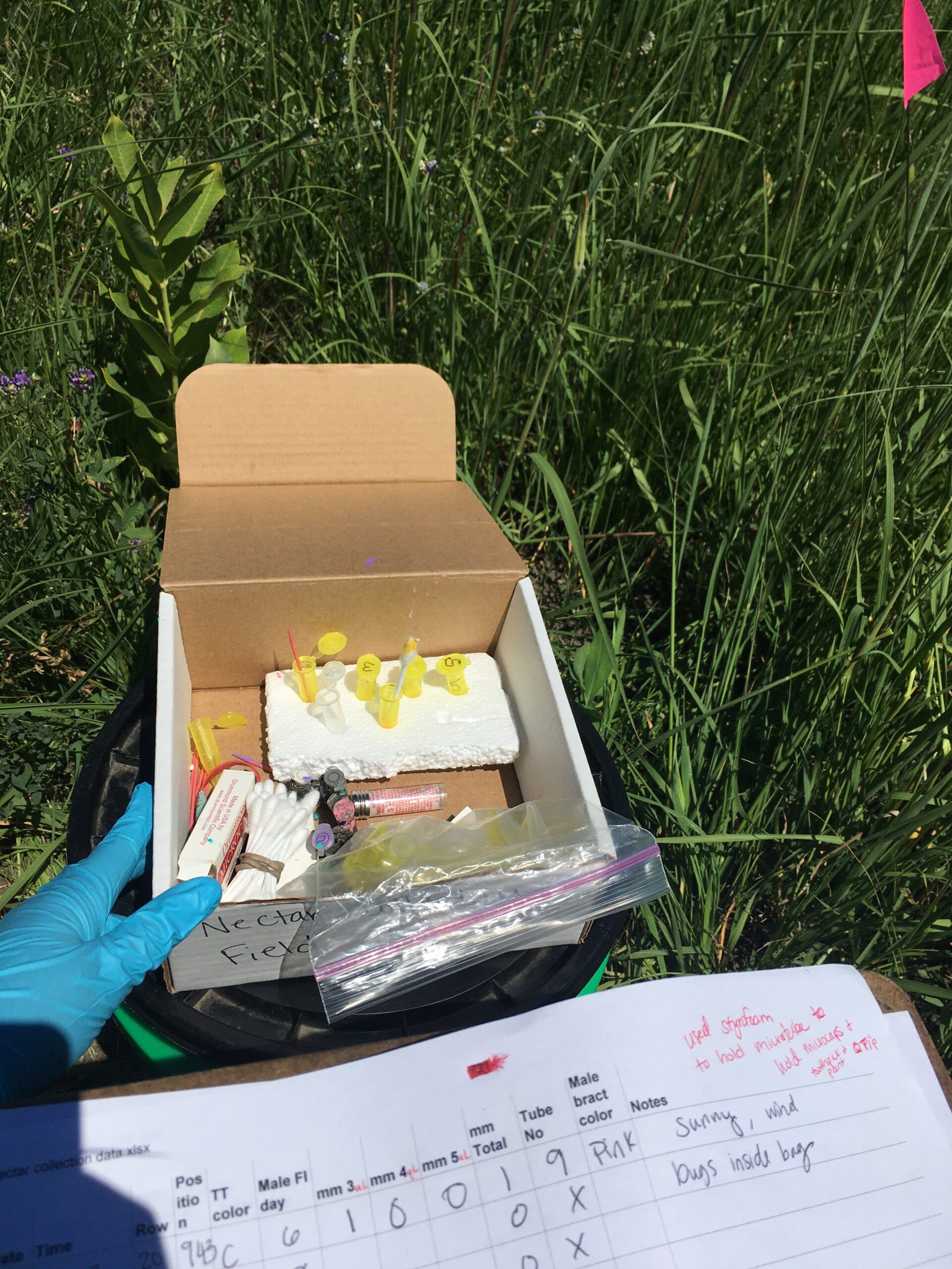
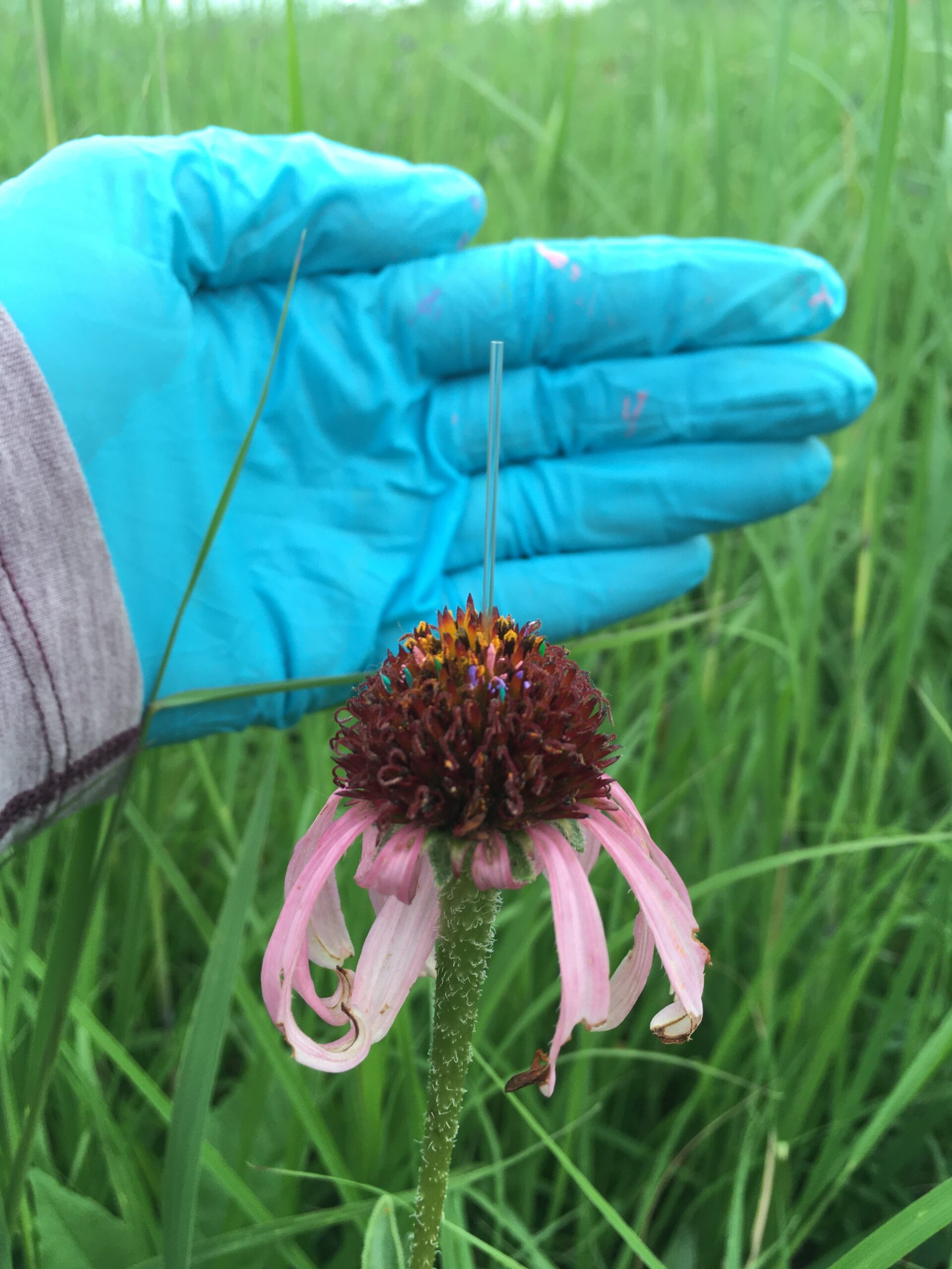
Me with the sweet magnifying glasses.A visitor in P1The must have equipment. Lots of pollen and painted bracts. I painted the bracts when I would come back to sample the same head so I would know which ones had already been sampled. First day, learning how to get it organized for easier collection. A more organized nectar collection field box.A microcap inserted into an anther.
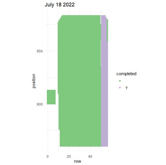
Last Friday (June 15th), the crew began measuring Echinacea in our largest experimental plot, P1! This plot has 10,673 positions that we visit during the summer, so it is no small task. We had 4 teams measuring for about 3.5 hours and visited about 1,471 positions (13.7% of the entire plot!). Above is a map indicating our progress, with purple representing the segments completed.
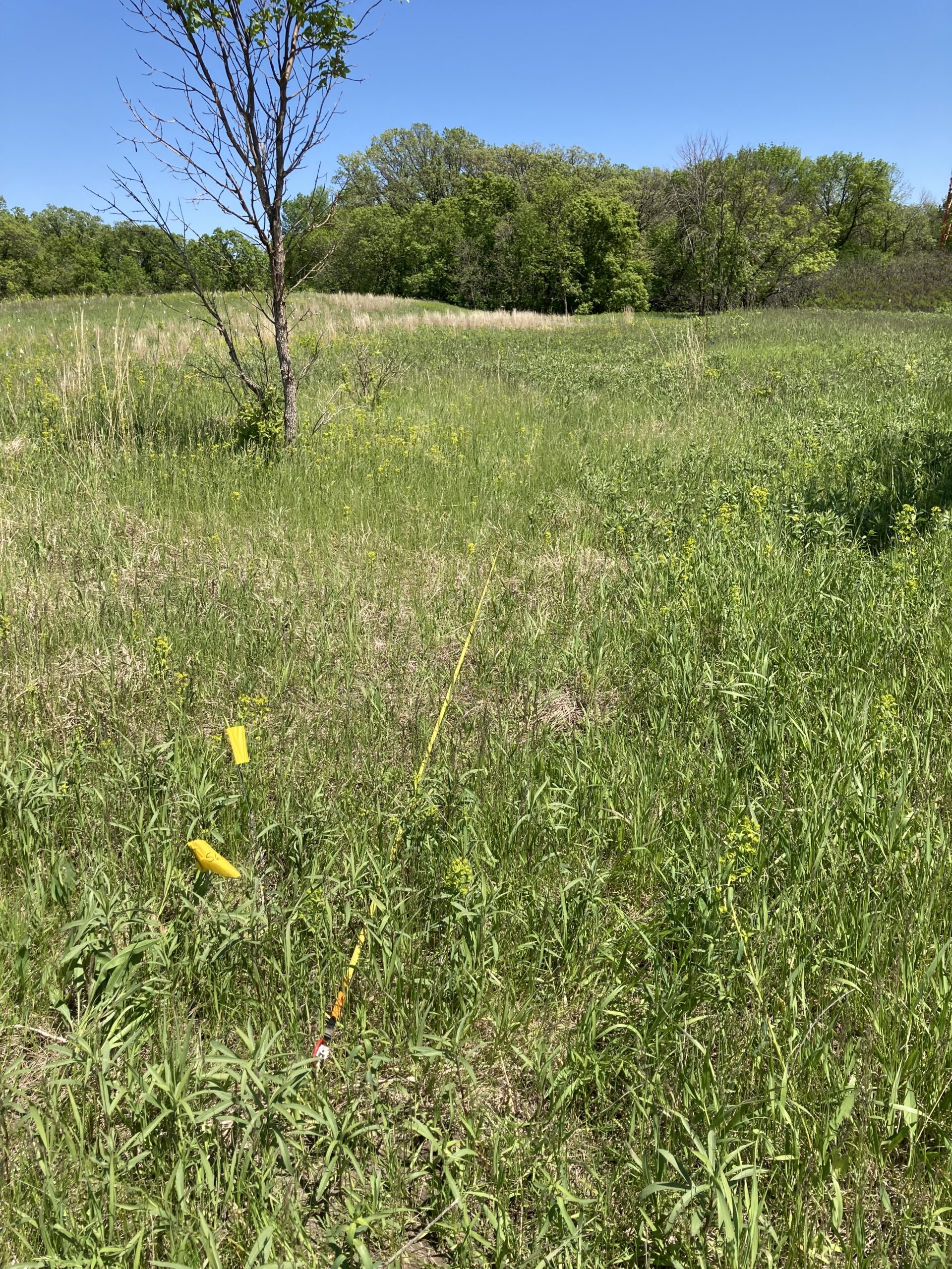
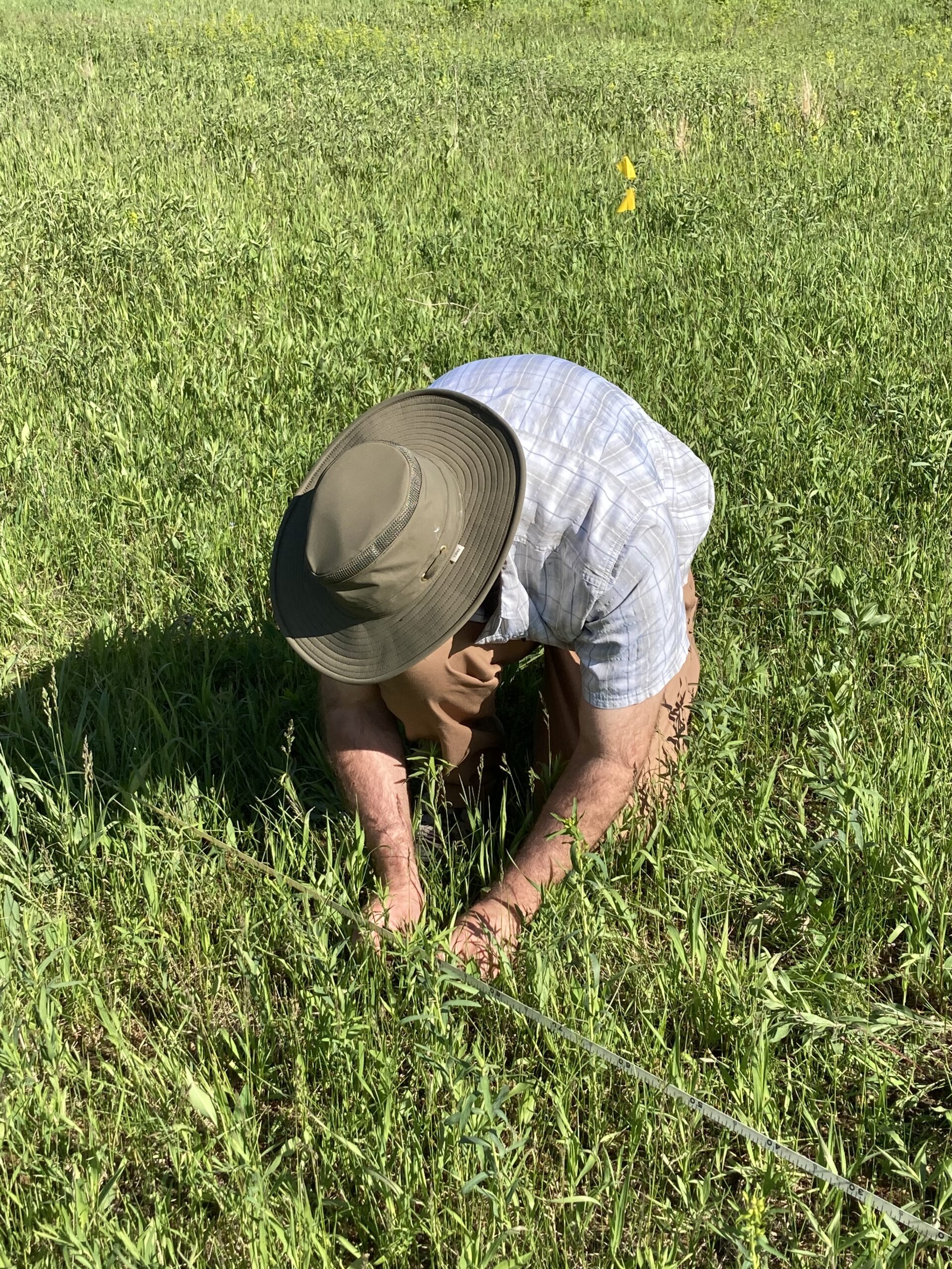
Between June 3 and June 12 (2022), members of the Echinacea Project planted 503 Green Milkweed (Asclepias viridiflora) seedlings across four sites in Solem Township. These sites included an area south of Experimental Plot 8 (149 seedlings planted June 3), a hilltop at Hegg Lake WMA (117 seedlings planted on June 9), a disturbed area at Staffanson Prairie Preserve (117 seedlings planted on June 10), and a hilltop at Eng Lake WPA (aka eth, 120 seedlings planted on June 12).
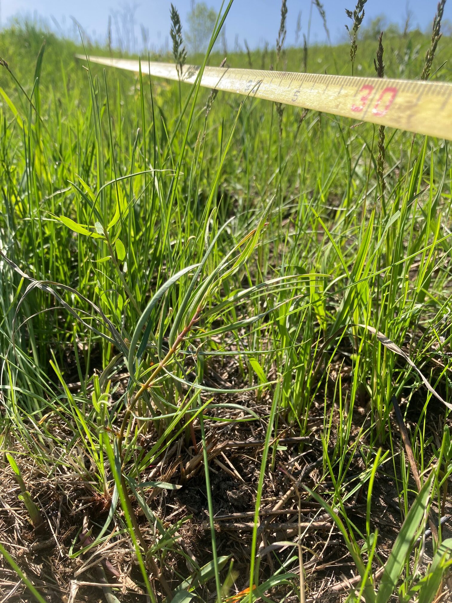
I promise this photo contains a green milkweed seedling we planted…
We hope these seedlings grown from locally-collected seed will establish new thriving populations of this declining plant species and provide a reliable seed source for future restorations. They may even provide future research opportunities to learn about the reproductive biology and demography of green milkweed! Thanks to the MN DNR, the Nature Conservancy, and USFWS for giving us permission to plant seedlings.
Attached is a csv containing the coordinates for parasitic plantings in exPt01. ID is a unique ID to a Row x Position combination, Row is the row in exPt01 (starts at row 13 and increases by 5), Position is the position in exPt01 (starts at 861.85 and increases by 5), Treatment is what was placed there (seeds, Comandra, Pedicularis, or C + P which is Comandra and Pedicularis), siteOne is where the first plant planted came from and siteTwo is where Pedicularis came from if Comandra and Pedicularis were both planted.
Last summer, we located 71 Asclepias viridiflora (green milkweed) plants in the remnants, and we collected pods from 22 plants. We brought the seeds back to the Chicago Botanic Garden, where Cathy Thomas propagated them at the production greenhouse. We were hoping for 392 milkweed seedlings, but the seeds germinated better than expected, so we now have 505 baby milkweeds!
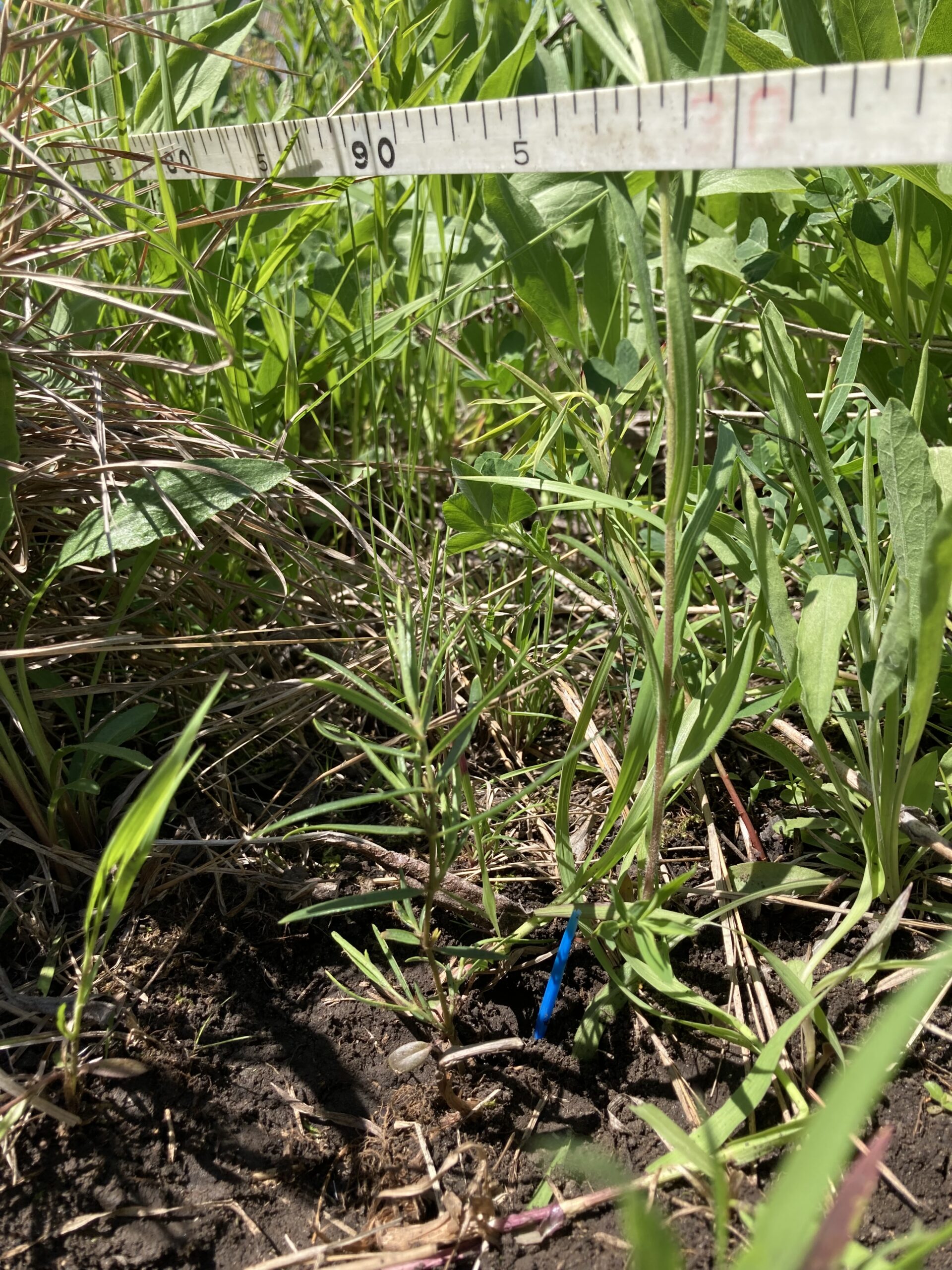
On Friday, Jared and I planted 149 Asclepias viridiflora plants south of p8. These plants represented 13 maternal lines. We flagged out five 30-m-long transects. Two transects are partially within the west Andropogon pilot plot, and three transects are partially within the east plot. Along each transect, we dug holes with soil knife 1 m apart, watered the holes, and planted the Asclepias plugs. We placed a toothpick 2 cm north of each plant and recorded the toothpick color. We were glad that we decided to add toothpicks; when I returned to water the milkweed plants, they were already nearly impossible to see!
Good news on the Liatris front: all hands-on work, from harvesting to x-raying, is complete! The process began in the summer of 2021 and involved lots of help from the field crew, wise, long-term Team Echinacea members, eager and efficient short-term members, and everyone in between.
Mia V and I were also able to complete data entry and data cleaning today, paving the road forward for analysis.
Now that we’re moving on to computer work, we came up with some primary questions to pursue (and some hypotheses):
Is there a significant difference in seed predation rates between burned and unburned and unburned remnants?
We suspect that predation will be higher in burned remnants because density of plants will be higher
Is there a correlation between seed predation rates and plant density?
We hypothesize that higher density will be correlated with higher rates of predation
We will use nearest neighbor as our measure of density
Is there a correlation between individual plant size and predation rates?
We hypothesize that larger plants will receive higher rates of predation
We will use number of flowering heads as our measure of plant size.
I’m now in the process of making plots to help us visualize the data we’ve collected, and soon we can begin to seek answers for our questions.
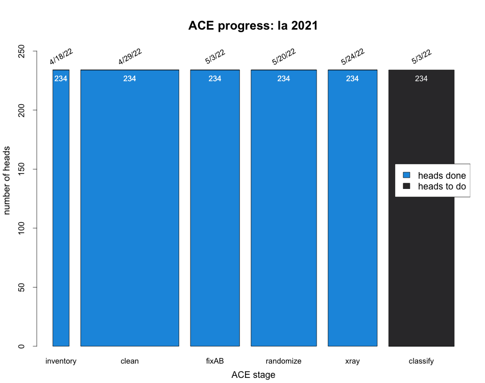
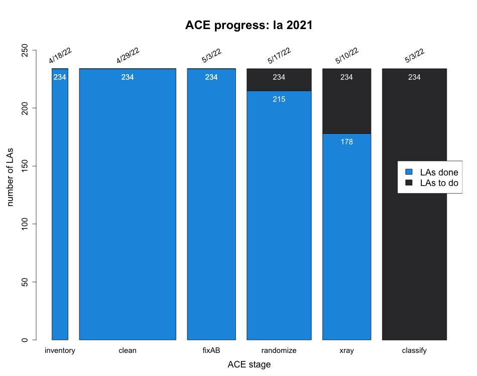
Because none of our questions at the moment directly relate to pollination, we don’t need to quantify seed set, which is the “classify” step. Using the x-rays to count how many achenes contain seeds is our method of determining pollination rates (seed = pollinated, no seed = not pollinated). This step will likely stay low priority for awhile, so don’t fret about the empty bar. All part of the plan.
Liatrisaspera 2021 progress in the lab is steadily marching on. Thanks to the work of the Carleton externs last winter, we began Northwestern’s spring quarter essentially halfway done (only needing to do some brief back-peddling due to a change in protocol).
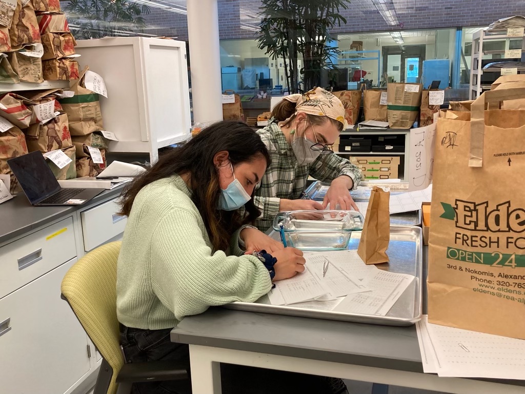
With the help of work study Mia V., cleaning, the process of removing the achenes from the flowering heads and gather data on achene-per-head count, is completely finished. Mia has also made excellent progress on randomizing, the step where we select a random sample of achenes to be x-rayed as well as quantify seed predation. We’re on track to finish randomizing later this week or next. Following that, we can x-ray the final batch of 56 liatris, allowing us to quantify seed set, and all the hands-on work for our 234 liatris from 2021 will be complete!
Mia and Wyatt cleaning Liatris aspera in the lab
Priorities going forward:
Finish randomizing and x-raying for batch D
Complete randomization data entry and verification
Develop methods of data analysis to compare
Burned vs. unburned predation rates
In regards to density
In regards to number of heads per plant
Develop methods of classifying seed set from x-rays (low priority)
To kick off our 2022 burn season, we conducted a prescribed burn in our eastern pilot Andropogon experimental plot on Friday, May 6. We burned the western plot in spring 2021.
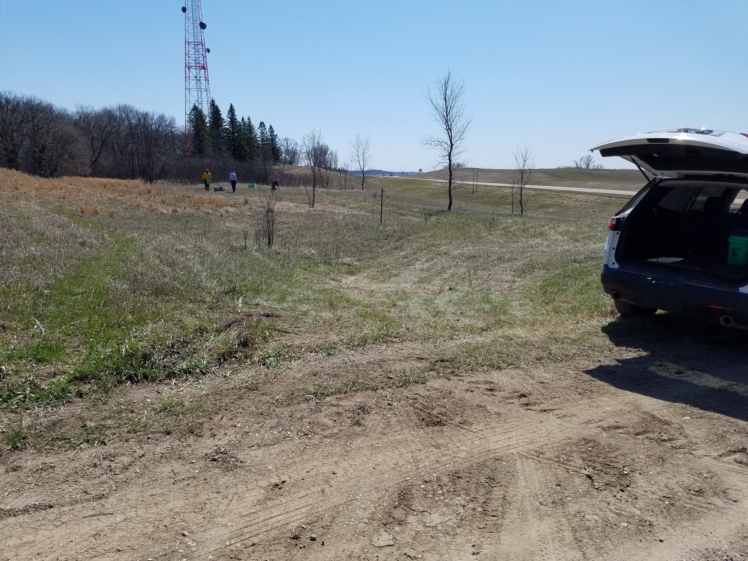
After staging equipment and checking the weather with our new bluetooth-enabled Kestrel, we ignited a test fire in the NW corner of the plot. The fire looked great and out mowed break was doing its job so we proceeded with the fire. Stuart kept watch over the northern line while Alex and Trygg tended to the western edge. We allowed the fire to back downhill against the wind. After putting in a few strips to quickly widen the black, we ignited along the eastern and southern lines. The headfire quickly ran uphill. Apart from areas with discontinuous fuels along the northern edge, the burn was pretty thorough. Stuart noted that the wind was consistently southeast except for a southern push when we ignited the headfire. We agreed that lighting the headfire sooner would have been possible given conditions and the fire behavior we observed. All-in-all, a successful first burn of 2022 for the Echinacea Project. We are eager to learn how Andropogon gerardii responds to fire.
Staging equipment for the burn (Stuart’s photo)
Stuart’s view of strip fire from the NE corner (Stuart’s photo)
Jared and Trygg keeping an eye on the western break (Alex C.’s photo)
Alex C. tending to the southern break as the headfire runs uphill.
Temperature: 65 F Relative Humidity: 37 % Wind Speed: 13 mph Wind Direction: SE Ignition time: 12:03 PM End time: 12:24 PM Burn Crew: Jared, Stuart, Alex C., Trygg
The lilium project is almost wrapping up as I am approaching the end of my semester long internship. I am almost finished with processing my seed data. All the scans and x-rays of lilium ovules have been done. The only steps left are to finish counting and classifying the ovules. Counting is done to quantify the total number of ovules in the each lilium pod. Classifying is using the x-ray image to determine the number of fertilized ovules in each pod. Once I have the data for the total and full counts of each lilium pod, I will be able to obtain the seed set for each individual lilium philadelphicum. Then, I will analyze the relationship between variation in seed set and proximity in nearest neighboring plants. Jared showed me the FNN package in R which, like its name, will find the nearest neighbor between x and y coordinates. The knn.dist function is a handy tool that allows you to compare distances of a point and its nth neighbors. In order to further analyze the data, my first step is to conduct data management and organize the different variables into a data frame. This process is very useful for researchers that use R for data analysis and data visualization. Next week, I will have a data frame that includes the information necessary for the analysis and visualization of the lilium data.
For the remnants, I finished data reconciliation for all the plants at Staffanson Prairie Preserve (spp) through 2021 in demap, our repository for data from the remnants. Each summer, we use the GPS to record the positions of every flowering Echinaceaangustifolia plant within the transect at Staffanson, and we also revisit plants that flowered previously to check whether they are still alive, a process called total demo. This winter, I connected records between years so we can track the life of individual plants across the years.
Last week, I completed demo.out for Staffanson in 2017, 2018, 2019, 2020, and 2021. Demo.out makes one record for each plant that we visited each year and records whether it was living or dead, whether it flowered, and how many heads it had. This is the dataset that we can use to do longitudinal data analysis and study the demography of Echinacea plants over time. In 2020, both sides of Staffanson burned, and it had the highest flowering rate in the past 5 years – 275 plants! Of those plants, 33 flowered for the first time. In 2021, there was just one new flowering plant.