|
|
Today started on the porch. We gathered at the table and talked about the tasks at hand. The first order of business involved organizing the mapped GPS data. Maps of all the remnants needed to be checked for missing GPS points and tag errors. Next up was an R Lesson. I loved learning the basics of loading/correcting data and executing a basic statistical test. After the morning lesson, we headed out to do a bit of GPS-ing and phenology at a few remnant sites, then gathered on the porch again for lunch.
After lunch, we started by pulling invasive thistles out of p1. After walking all the rows, we pulled 117 thistles in total! The two most impressive pulls were giant roadside plants seen below.
 Matt’s huge thistle!  Danny’s bouquet
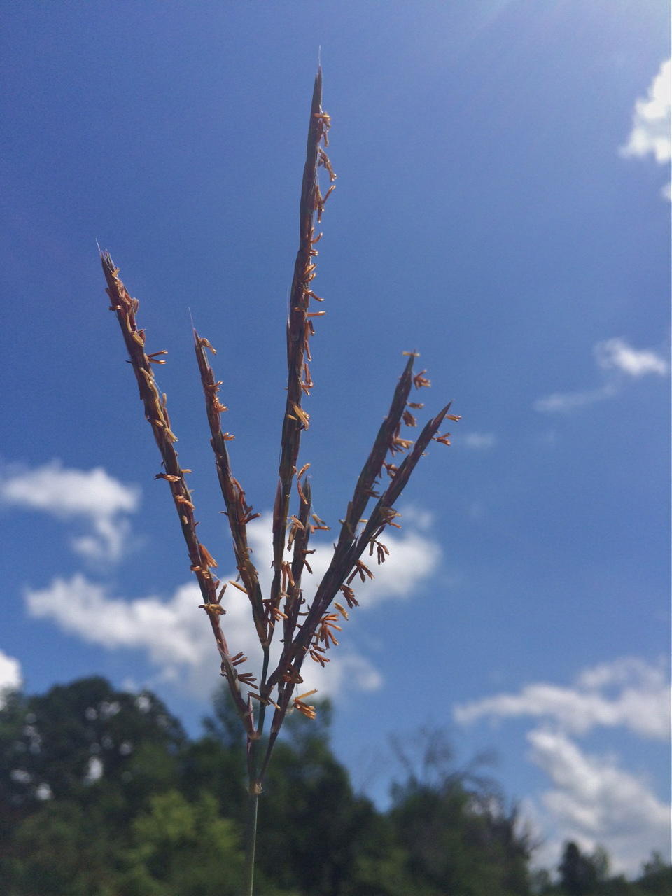
After the thistles were pulled, we moved on to hand crossing heads for Q3. On the way out to cross, I noticed some flowering grasses!
 
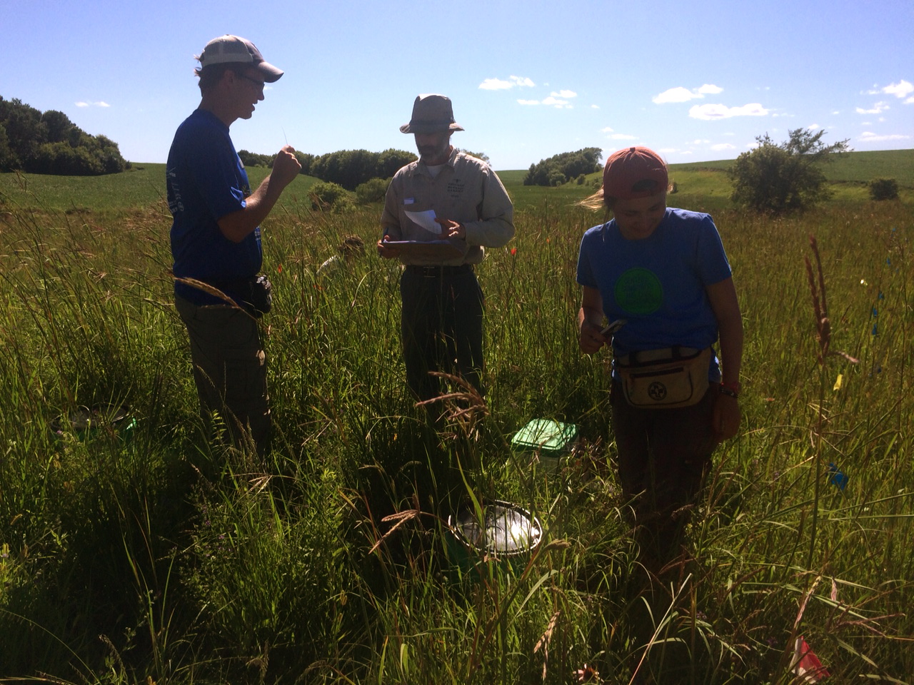
Staffanson pollen was organized and put into insulating styrofoam containers that correspond to each data sheet. We worked consistently until all 28 data sheets were complete, and all heads crossed.
 Crossing is almost done!  Stuart passes out pollen.
The days and weeks are starting to fly by as we get into the busy part of the summer. Nearing the end of July, it seems like we’re hovering right around the peak of the flowering season for Echinacea angustifolia. In addition to keeping up with the phenology for our flowers (roughly a couple thousand across our remnants alone!), we’re also making timely progress on independent projects and getting important work done on the q3 experiment.
We got off to a quick start this morning sending half the crew out to do phenology at a handful of sites while Danny and Amy continued their work assessing compatibility across remnant flowers and still a few others collected pollen at Staffanson for q3. While phenology is proving to be quite the time commitment right now, we’re slowly (and satisfyingly) starting to be able to check the “Done flowering” box for more and more of our flowers. The flowering season is tapering off much faster than I had expected!
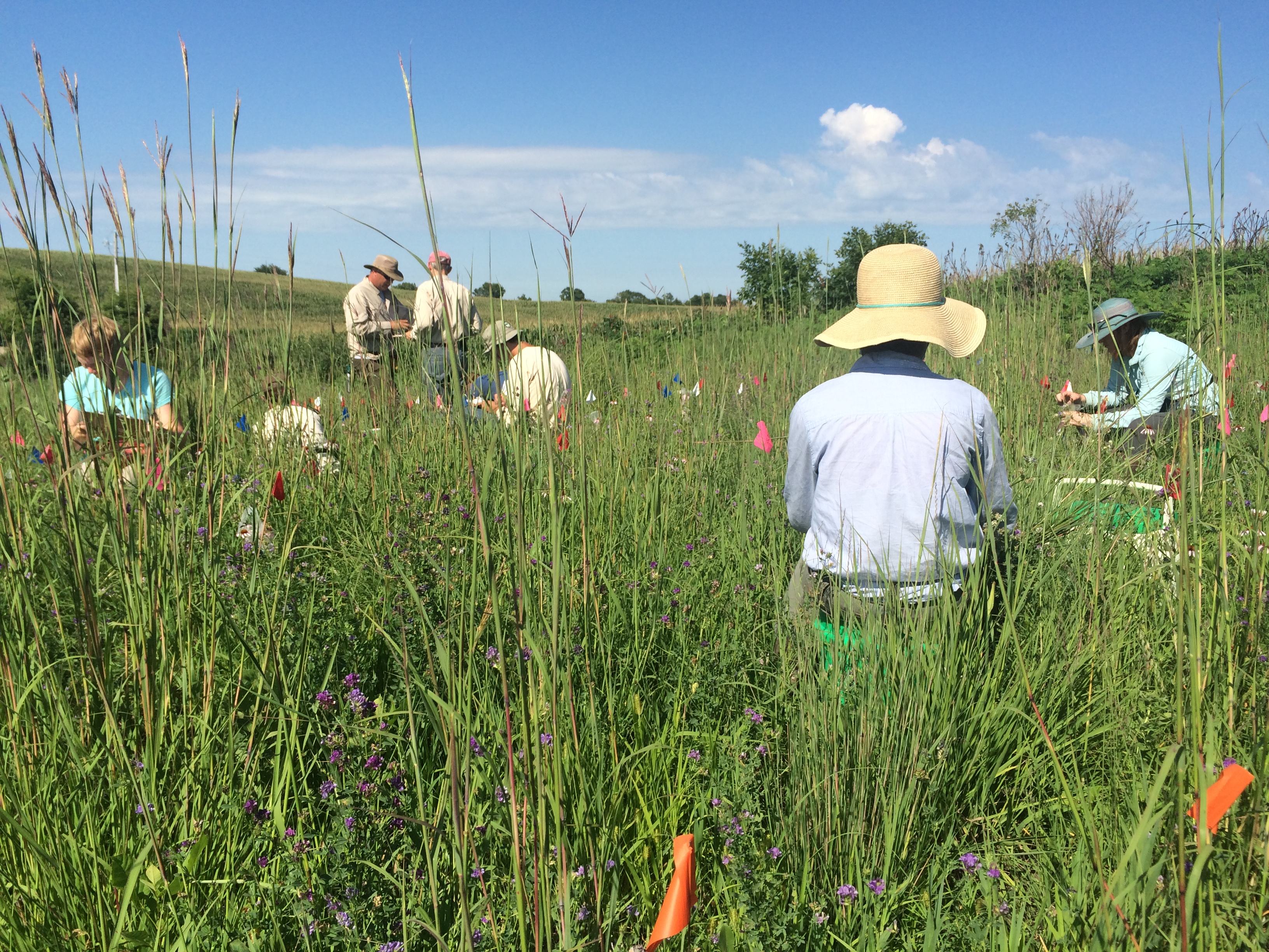
 A cross-pollinator’s eye view of a well-organized team carrying out crosses in p1. The bright and breezy afternoon had most of the team out in p1 doing pollen crosses for q3. Stuart debuted a new system for keeping us organized in the field as we share, swap, switch, and track down the right vials of sire pollen to be applied to the p1 dams. While the fits of wind that persisted for much of the afternoon were a nice way to cool down, it was not very much appreciated when the breeze swept away the valuable bits of pollen we were trying to apply to our flowers!
The day ended with a visit from some of the parents of the crew members and local science teachers (these two groups actually had quite a bit of overlap). These visits were timed excellently for our guests to appreciate the Echinacea in all their peak flowering glory.
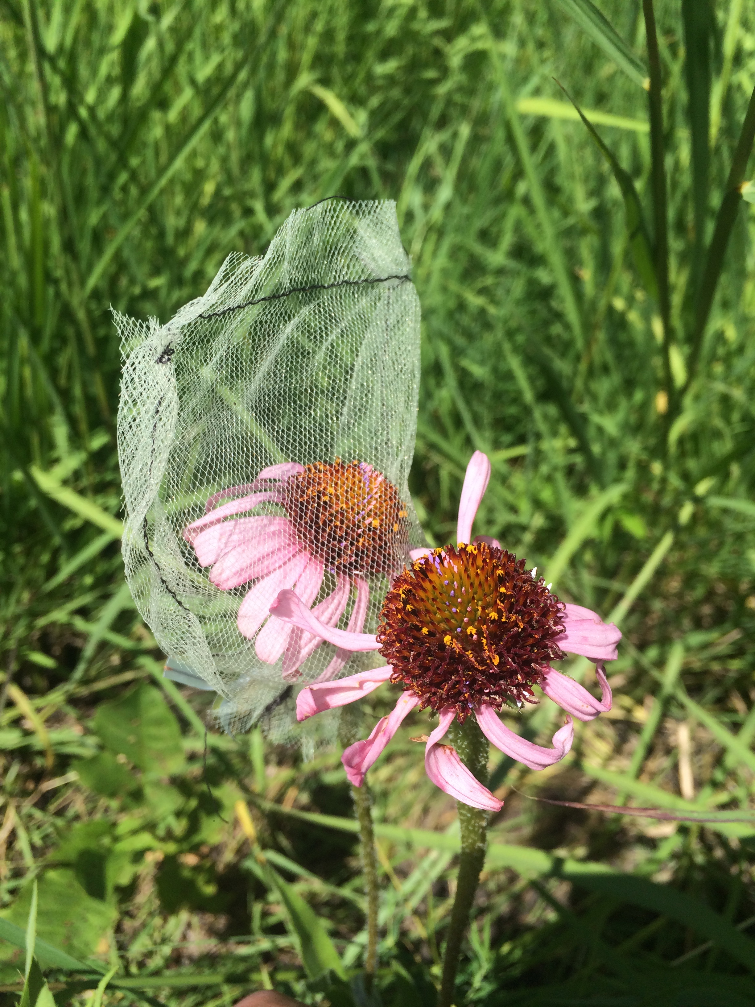
 Bagged and painted Echinacea ready to be cross-pollinated.
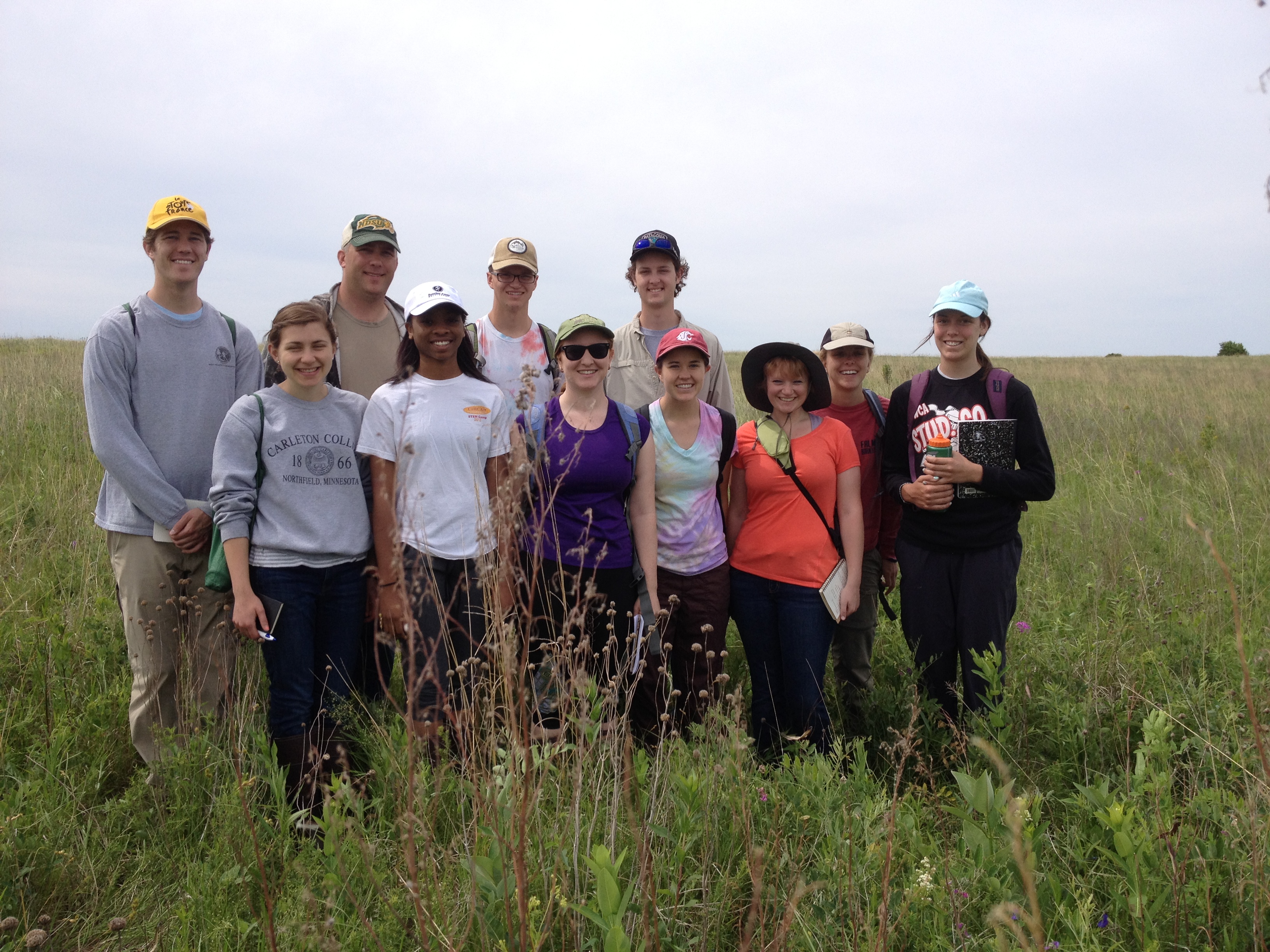
The summer field season is off to a great start! We have assembled an excellent team to investigate ecology and evolution in fragmented prairie habitat focusing on the narrow-leaved purple coneflower as a model organism. Meet members of the team.
Team Echinacea 2015: Danny, Matt, Ben, Will, Gina, Taylor, Lea, Amy, Katherine, Alison, Abby
We started the season with tours of local prairies large and small, including Staffanson Prairie Preserve, Hegg Lake WMA, which are large and protected. Stay tuned for team-members’ first impressions of some of the nearby remnant Echinacea populations.
Team-members hail from near & far: Barrett, Elbow Lake, and Alexandria, Minnesota & California, Alabama, New York, and Rhode Island. They are excited to develop summer projects and they will post their proposals here next week. Our team includes four college students, four who just graduated college, two high school teachers, and one high school student. And there are the old-timers.
To get ready for field work, we took the Hjelm House out of winter storage and cleaned out our storage facilities (g3). We inventoried supplies and made signs and tags for fieldwork. Everyone got a pouch with tools and supplies and Gretel has assigned us all a data collector. This may be (should be) the last year for our trusty handspring visor data collectors. The visors are trustworthy, but the computers and software that run them are showing their age.
The first main activity of the season was assessing survival and growth of 2526 plants in the Q2 experiment, which is designed to quantify the additive genetic variation in two Echinacea populations. The amount of additive genetic variation determines a population’s capacity for adaptation by natural selection. Genetic variation is very important for the persistence of populations in prairie habitat. We’ll find out how much variation Echinacea has, which will give us some ideas about future prospects for these populations in the rough-and-tumble and rapidly changing world out here.
We got rained out several times this week, but managed to measure all 2526 plants. We found a few plants that escaped detection last summer and we even found one seedling. Welcome to the experiment, fellas! We’ve got our eyes on you.
Overwinter survival appears to be quite good and most of the toothpicks we used to identify individual plants made it through the winter too. The tallest plants were just over 20 cm and some plants had 3 or more leaves. This is great news for plants that were sown as seed in fall 2013. Growth conditions are challenging: a cold winter with little snow, a dry spring, shading out by established plants, chewing by herbivores, … it’s a tough life for a prairie plant.
All in all, it promises to be a great summer. We’ll keep you posted.
Dwight and Stuart broadcast native prairie seed in experimental plots p1 & p8 on Friday. At 34 °F (1°C) it was the warmest day in a month. It was also very windy –great for spreading seed! We broadcast Bouteloua curtipedula, Schizachyrium scoparium, Galium boreale, and Phlox pilosa directly on the snow. There wasn’t much snow and it was melting. We broadcast Lathyrus venosus in p1. We stored about half of each species, except L. venosus, in the Hjelm house to broadcast in the spring. (Hedging our bets.)
Experimental plot 1 (P1) encompasses 11 different experiments originally planted with a total of 10673 Echinacea individuals. These experiments include long-term studies designed to compare the fitness of Echinacea from different remnant populations (“EA from remnants in P1”), examine the effects of inbreeding on plant fitness (“INB” and “INB2”), and explore other genetic properties of Echinacea such as trait heritability (“qGen”). In 2014, Team Echinacea measured plant traits for the 5409 Echinacea plants that remain alive and followed the daily phenology of 567 flowering heads. Echinacea began producing florets on July 1 and continued flowering in P1 until August 24. The data collected in 2014 will allow us to estimate the heritability of various traits and assess the lifetime fitness of plants from the numerous experiments.
|
Experiment |
Year planted |
# alive |
# flowering |
# planted |
| 1 |
1996 |
1996 |
314 |
115 |
650 |
| 2 |
1997 |
1997 |
270 |
57 |
600 |
| 3 |
1998 |
1998 |
32 |
3 |
375 |
| 4 |
1999 |
1999 |
542 |
106 |
888 |
| 5 |
1999S |
1999 |
297 |
37 |
418 |
| 6 |
SPP |
2001 |
318 |
14 |
797 |
| 7 |
Inbreeding |
2001 |
221 |
15 |
557 |
| 8 |
2001 |
2001 |
170 |
11 |
350 |
| 9 |
Monica 2003 |
2003 |
28 |
3 |
100 |
| 10 |
qGen |
2003 |
2501 |
122 |
4468 |
| 11 |
INB2 |
2006 |
716 |
41 |
1470 |
Start year: 1996
Location: experimental plot 1
Products:
Overlaps with: aphid addition exclusion, Pamela’s functional traits, pollen longevity, pollen addition exclusion
We started out the day doing what we do best: searching for seedlings in Experimental Plot 8 (a.k.a. Q2). Having braved formidable winds to plant them late last October, Stuart, Gretel, and Ruth were visibly relieved to see them pop up this spring. Since last week Team Echinacea has been diligently tracking down each seedling and “naming” them with colored toothpicks and row location coordinates, accurate to one centimeter.
In the afternoon we located and counted Echinacea in the recruitment experiment, a continuation of the project described in this paper. The procedure is really fun: we find the boundaries of the plots with metal detectors, triangulate points, then search within an area exactly the size of a regulation 175-gram Disc-craft Ultra Star disc (a.k.a. frisbee). Go CUT!
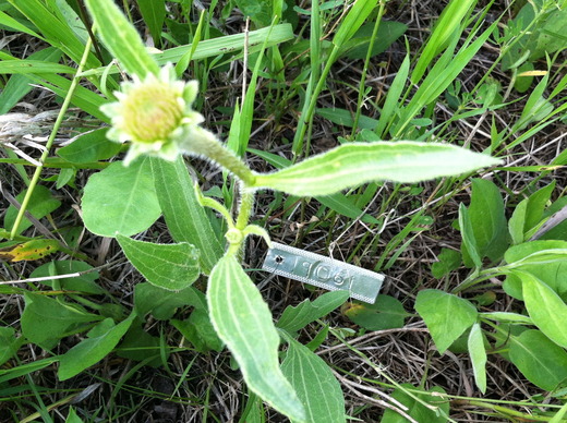
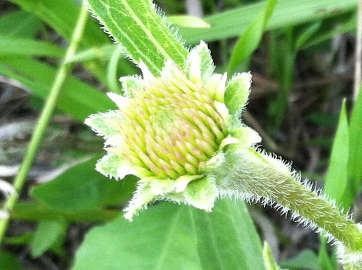
The best part of the day was tagging my first Echinacea. Maybe it just lost its old tag, but I like to think this is the first time this plant has ever born the silver badge. Sometime 10-12 years ago, this seed was planted. Now that it is finally about to flower, it has the honor of going down in history in the databases of the Echinacea Project, living out the rest of its life in the service of science. This 23rd of June, 3.65 m from the southwest corner and 0.79 m from the southeast corner of the northeast plot in Recruit 9, I named a flowerstalk “19061.” Isn’t it beautiful?

Doesn’t the flower head look ripe? Stuart says we may start to see flowering as early as the end of this week!
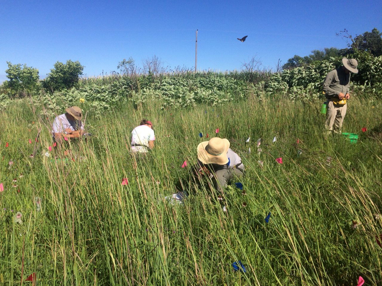
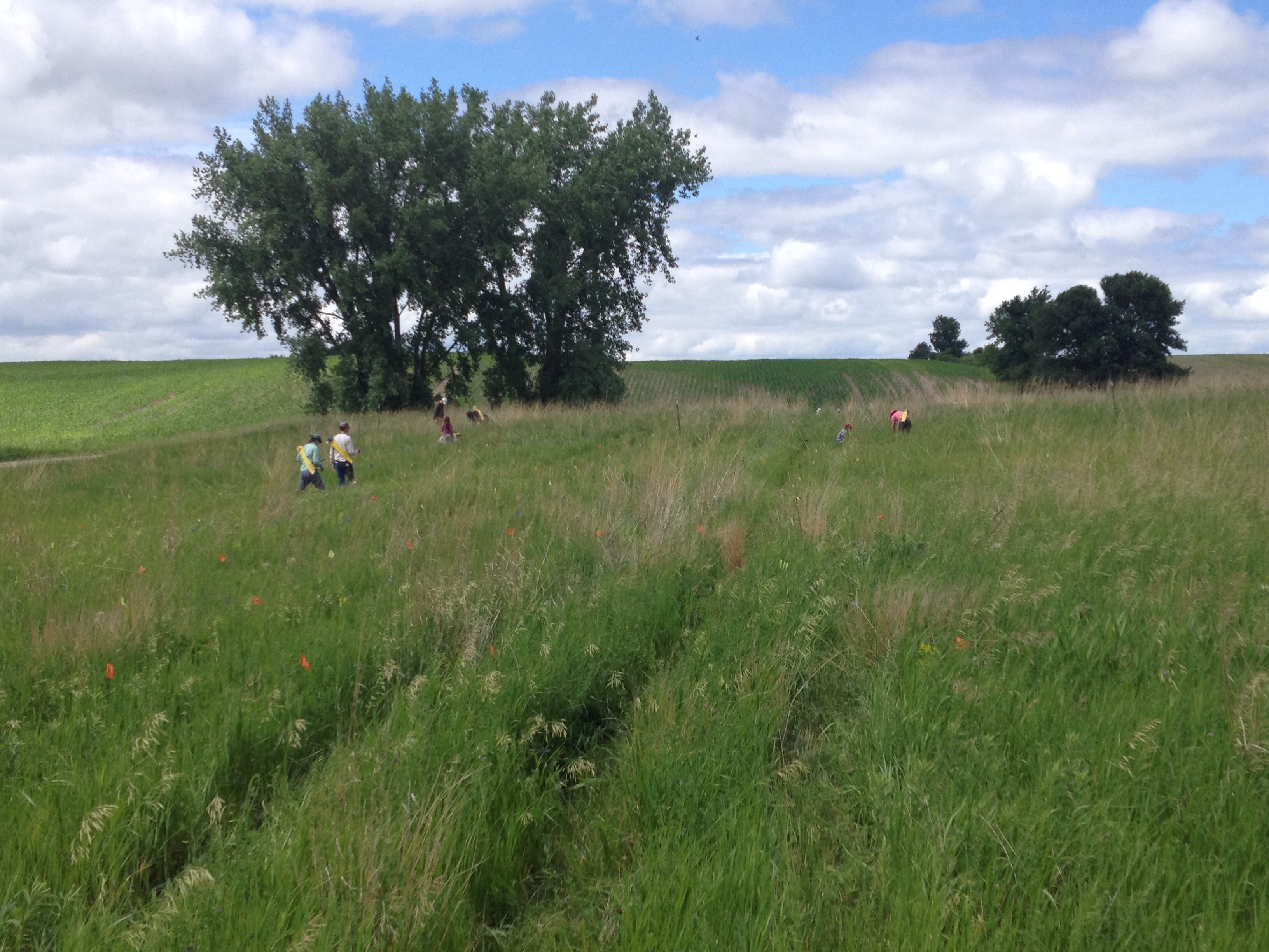
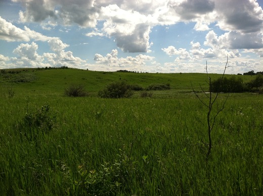
Eventually the time came to leave my new friend and join the rest of the team. This is where they were:
(Can you spot the team?)
A nice day is Douglas County is a very nice day.
We had a very quick and efficient planting last week. Stuart and I drove up to MN on Thursday morning, picking up Katherine Muller on the way in St. Paul. We arrived in Kensington on Thursday evening, and immediately got to work. We broadcasted our remaining little bluestem and side oats gramma grass seeds in the South Field (where we planted our qGen2 achenes this fall, aka CG-8). We walked E/W throughout the plot and each broadcast seed over a 5m area. We also broadcast seed around the edge of the plot. Here’s an inventory of how much we broadcast from each of the collection sites:
Peninsula – 1 quart
Back Hill – 1 quart
LCW – 2 quarts
CR-15 – 1 quart
Tower – 1 quart
Krus – 1 quart
RRX- 1 oz
CG1 – 1 gallon (24 Sept) + 1 gallon (30 Sept) + 2.5 gallons (2 Oct).
We then headed to Hegg Lake to scout out a planting site for the sprouts. We settled on a spot near the parking area, to the west of Amy’s, Caroline’s, and the recruitment plots. The plot is 12m x 30 m with 13 rows and 60 positions. There is a meter spacing between rows and half a meter between positions.
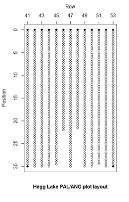
We returned the next morning and began planting by 9:30am. With three of us we were very efficient and finished our last row by 3:30pm. We we lucky to have beautiful weather, it was sunny all day with temperatures in the low-mid 70s and a consistently strong breeze. All positions in the plot were plant-able. Here’s a diagram of the plot:

Empty circles indicate positions where a sprout was planted and black dots indicate positions where there are nails. Plants begin at position 0.5 in every row. Row 41 is the most western row, and position 0 is closest to the road (and north). There are empty positions at the ends of rows 46 and 48. There is a bent over flag at each of the 4 corners of the plot.
I’m excited to have the sprouts in the ground and to have participated in my first planting. Fingers crossed we have high survival!
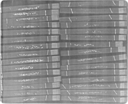
We took some high-quality images of Echinacea achenes for our q2 experiment this fall; an example is below. Notice how easy it is to distinguish empty achenes from those with embryos. By darkening the room and removing the opaque film, we were able to use lower levels of xrays for a shorter duration than we have previously. This plate was exposed to 12kV x-rays for 4s. We used long, thin glassine envelopes to facilitate counting. Notice also that the laser-printed labels reveal the packet IDs.

X-ray image of 30 packets of achenes from
Echinacea angustifolia. Click on thumbnail to enlarge.
We are preparing to plant a new experiment this fall. We are cutting down ash trees (Fraxinus pennsylvanicus) in an abandoned agricultural field that was planted with Brome in the 1980s. We will plant Echinacea angustifolia seeds from our experimental crosses this summer. We will hand broadcast two native warm-season grasses: Bouteloua curtipendula (sideoats grama) and Schizachyrium scoparium (little bluestem). Keep up-to-date on progress on this experiment via twitter.

Dwight, Lydia, & Ilse with tools of the day: chainsaw, loppers, brushcutter. Not shown: paintbrush.
|
|