|
|
(Aghh I just finished writing and then when i tried to publish the site told me that my session had expired and of course I lost the whole blog post T___T )
Anyways…
Today was a very hot and humid day. Temperatures into the 90s, feeling like 100. Sweaty sweaty sweaty.
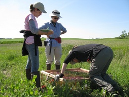
Some of us accomplished field work.
Andrew was in C1 this morning painting bracts and bagging Ech flowers.
Katherine was also in C1 doing her aphid add/exclude experiment.
Shona was out at Hegg Lake for 4 hours painting bracts and observing crossed styles.
I (Maria) was also at Hegg Lake (for my own reference from around 10.30 – 4.40pm) surveying Dichanthelium inflorescences I’ve been tracking for the past week or so, and more importantly, finding plants for my pollen limitation experiment. I have 31 plants flagged and 62 inflorescences twist-tied. I’ll be initiating the experiment tomorrow, so I should be in bed now (hence, I’ll give more details in a later post).
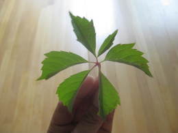
To end off the week, here’s a special 6-leaved Virginia Creeper (they are usually 5-leaved) I found in the 99 south garden. Hope it brings everyone good luck!

Here are the day’s events:
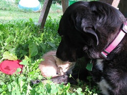
When we arrived at work this morning we came upon a poignant scene. The Wagenius’ family dog, Roxie, had was nurturing an abandoned kitten:
I’m happy to say the poor creature has found a home with Kelly and her parents. Thanks to her loving care (and Roxie’s), it is now purring and mewling with gusto.
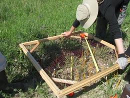
Once the kitty situation was resolved, we moved on to more serious business. Shona, Maria, Kelly, and Lydia spent the morning working on their individual projects while the rest of us assessed flowering phenology in two experimental plots (C1 and C2).
A lot of work goes into maintaining an experimental plot. In order to keep C1 from being overgrown by woody plants, several of us spent the afternoon trimming ash trees and sumac. The rest of us made progress on our individual projects. Thanks to help from Kelly and Lydia, Jill and I succeeded in setting up ant traps for all but one of our field sites. I’ll post more about that later.
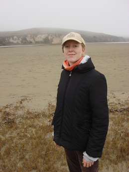
I don’t know if I’ve properly introduced myself on here.
My name is Katherine Muller and I’m a second year Master’s student at Northwestern. I hail from the lovely, temperate San Francisco Bay Area. I’m not sure whether it was my thirst for adventure or my contrarian nature that led me to the Midwest–first to Oberlin College in Ohio, then to Northwestern and Minnesota. In any case, I now have the privilege of complaining about the weather.
This is my second year with the Echinacea Project. Last year I began research on aphids and ants in Echinacea angustifolia. I have two projects that I plan to continue this summer:
My first project is an experiment examining the effects of aphid infestation on Echinacea. Last year, I selected 100 non-flowering Echinacea, excluded aphids from 50 plants and added aphids to the other 50. I am repeating the experiment on the same plants. I performed my first experimental treatments on Saturday and Sunday and should soon be able to analyze my results from last year.
The other project I plan to continue this year is a survey of aphids and ants in a large experimental common garden. Last year I selected a 20x20m section of the experimental plot and led a biweekly of ants and aphids. I started this because I was interested in seeing how aphids spread over space and time. This year I will examine the same area to see how aphid infestation changes from year to year. Thanks to everyone’s help, I collected my first dataset on June 15th. Considering the unusually warm winter, there should be some interesting developments this year.
My third project is to assess aphid and ant abundance among several Echinacea populations. My original plan was to survey aphids and ants on a representative sample of the entire population, including juvenile and non-flowering plants. As it so happens, Amy Dykstra and Daniel Rath conducted a similar survey in 2009 (you can read about it in the archives). For all their hard work, they found very few plants with aphids. Of the plants they surveyed–flowering plants had a much higher rate of aphid infestation than non-flowering plants–32% for flowering versus 5% for non-flowering plants. I decided to take a different approach and focus my sampling effort on flowering plants. Specifically, I will survey aphid and ant abundance on plants that flowered this year and last year. This will allow me to assess whether flowering in one year influences the likelihood of aphid infestation the following year.
That’s about it for now. I’ll be posting my progress on here as it happens. This summer I have the privilege of collaborating with Jill Gall, an REU student from College of the Atlantic. She’s been hard at work preparing her project assessing ant diversity in prairie remnants, which I’ll let her tell you about.
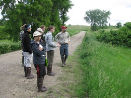
And because everyone else is doing it, here’s a picture:

Katherine here.
Most of the Echinacea crew arrived on Sunday. The week has gotten off to a running start. Here are some pictures from our first few days in action:
We just reorganized the bee collection into a cornell drawer, and need a cabinet to start storing drawers. Once we have better humidity control in the Hjelm house this is the cabinet we are considering.
cabinet
Hello everyone! This is Sebastian with another update on the x-ray machine. This post will discuss the various methods that can be used to determine the radiation dose of our x-ray machine. Below you will find my report on determining x-ray radiation doses.
Evaluating 3 methods for estimating radiation doses
23 March 2012
Sebastian Di Clemente
Introduction:
The population biology lab is trying to determine the dose of x-ray radiation that the x-ray tube emits per x-ray taken. Calculating the radiation dose is not an easy task because there is no straight forward way to do it. Each method used to determine the x-ray dose presents several differences in measure and calculation. Knowing the radiation dose of the x-rays can be used to determine what dose levels will hinder or harm a seed and what dose levels may even be beneficial to seeds; in short, knowing the radiation dose will allow researchers to quantify the point where seeds are affected by the radiation. With this experiment I will evaluate the sources that give the x-ray radiation dose and analyze the information given by each source.
Objectives:
1. To determine what method gives the most accurate information
2. To determine what method should be consulted to find the most appropriate radiation dose
Methods:
I gathered information based on web searches, contacting professionals, and contacting the x-ray machine manufacturer. I 1.) found a web page that calculates the x-ray radiation dose level and 2.) the manufacture provided the information that they have on dose levels that the Faxitron MX-20 machine produce at various settings. After receiving this information I test the web calculator by inputting the same settings that the manufacture provided and then compared the calculator reading to the value given by the manufacturer. I also further examined the information that the manufacturer provided and determined any differences in information or information format. The use of 3.) a dosimeter would give the most accurate measurement.
Results:
After comparing the web calculator result to the information given by the manufacturer using the same settings and criteria there is a significant difference in the dose level given. The web calculator had a dose level that was greater than the valued indicated by the manufacturer for lower level voltages (less than 20 kV), but the manufacturer indicated a greater dose level at anything above 20kV compared to the web calculator. The professionals offer the solution of a dosimeter. The comparison of the manufacturer data to the web calculator, and the three methods are provided in table below.
Comparison between manufacturer data and web calculator:
View image
The web calculator:
http://www.radprocalculator.com/XRay.aspx
The information given by the manufacturer is given in the following documents:
Dosage MX 20.pdf
mx-20 EXPOSURE DATA.pdf
MX-20 mR Ouput versus time.pdf
The professionals offer the solution of a dosimeter.
Conclusion:
Considering all of the information that I gathered I would trust the manufacture data over the web calculator data. The web calculator is good for fast calculations and changing between what units the dose level will be expressed in. Although, after testing the web calculator and see such a significant difference between it’s calculation and the manufacturer data, I feel that the manufacture would be more likely to have more accurate information.
Since the manufacture data is most reliable it is the clear choice to use. The manufacturer data covers more information, such as time, voltage, as well as unit conversions for other factors. Considering that more information is provided more variations to experiments can be made and the radiation does would still be available after simple unit conversions.
The other option presented by professionals would be to use a dosimeter to directly measure the radiation dose. This option would be the easiest way out of the three options, and would cater more to a researcher’s specific setting. If a dosimeter is available to use I would make this device my choice for determining radiation dose.
Hello Project Echinacea Flog!,
My name is Sebastian Di Clemente I am the Lake Forest College 2012 spring intern class of 2013, and I am quite excited about, this, my first post. I’ve been assigned the project of determining the best settings and magnifications for the new x-ray machine. Below you will find my report about the various magnification levels.
X-ray machine magnification
27 February 2012
Sebastian Di Clemente
Introduction:
The population biology lab is trying to determine the best x-ray magnification to use for scanning Echinacea achenes. The criteria that constitute “best” are image quality and contrast, label legibility, and overall time and efficiency. Each magnification presents different advantages and disadvantages, some more prominent than others. The use of these x-rays can give a more definitive answer of whether an achene has been fertilized compared to achene weight. With this experiment I will evaluate the x-ray machine magnification levels and determine the best choices and ideally isolate one magnification setting that would be best.
Objectives:
1. Obtain the best contrast quality possible for achenes
2. Obtain the best quality setting to read the label on the envelope
3. To determine the best settings and magnifications to use to maximize both label legibility and achene contrast
Methods:
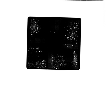
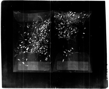
I scanned batches of Echinacea achenes in envelopes under the 10 second and 18 kv setting on the x-ray machine at the varying magnifications (magnifications are 1:1; 1:1.5; 1:2; 1:3; 1:4; 1:5) and window level settings. After taking a number of images at each magnification and assigning the prescribed window level settings (see X-Ray Machine Protocol for Echinacea) I compared images side by side. I then documented similarities and differences, and pros and cons of each image on their own and in relation to the other images taken. Based on the resulting images and my notes, I determined what each magnification might be useful for. Finally, I choose two magnifications out of the six that I thought would be most useful, and then weighed the pros and cons of each one more heavily and made my final choice as to which magnification would probably be best.
Results:
1:1 Magnification

At the 1:1 magnification the labels are hardly visible. The zooming in on this image would not do that much good because the image will become more pixilated. It is quite difficult to distinguish the achenes that are hollow and have not been germinated. Also, it is not possible to tell where the envelopes end or begin. The only real benefits of this setting are that four envelops can be scanned at a time and the achenes that have an embryo can be fairly easily counted.
1:1.5 Magnification
A magnification of 1:1.5 clearly does not show the greatest image. Although three envelopes can be captured in the image the labels are rather difficult to read and part of the third envelope gets cut off. The orientation of the envelopes is also a bit confusing and more laborious to set up. Positives of the image are that a large sample of achenes can be processed at a time. Another benefit is that after zooming in on the picture the achenes are easy to count and the visibility of germinated and non germinated achenes is fairly clear.
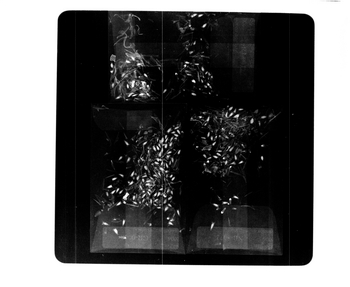
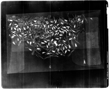
1:2 Magnification

The first benefit the 1:2 magnification has is that two envelopes can be scanned at a time. This benefit can double the speed of the scanning process. The extra space around the two envelopes can be use to include any smaller envelopes that may come inside the main envelope. The labels in this setting are still readable and the achenes show up nicely. The image needs to be zoomed in upon to provide a more accurate count of the achenes and to tell which have been germinated and which have not. If time is not of the essence, one of the magnification settings soon to follow would be recommended.
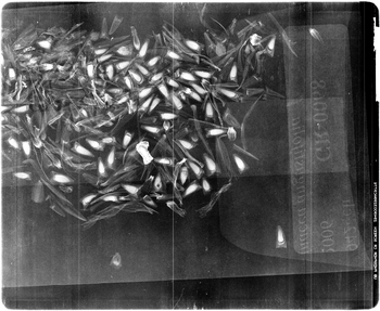
1:3 Magnification
The magnification setting of 1:3 is a good compromise between the previous settings and the settings to soon be discussed. This setting provides an image that encompasses a full envelope and leaves some room to spare. The extra room can be used for adding any small envelopes used to set aside certain achenes that may come inside the main envelope. The label in this image is fairly legible and every achene can be counted. It is also possible to determine which achenes have an embryo or are lacking an embryo. Furthermore, if the image is zoomed in upon it is possible to see any damage or defects of the achenes. The only issue with this magnification setting is that only one envelope can be scanned at a time, which makes the overall scanning process proceed at a slower tempo.
1:4 Magnification
A 1:4 magnification setting provides a fine image that shows both the label and the achenes clearly. From this magnification it is easy to count achenes, see any damage or defects of achenes, and tell whether achenes are hollow or have an embryo. Drawbacks to this setting are that the entirety of the envelope is not captured in the image, which leaves achenes not visible at the bottom or top of envelop that is cut off. Another obvious set back is that it is only possible to view one envelope at a time. This setting would be recommended to use if a close examination of the achenes is need, especially when trying to examine a greater number of achenes at a time.
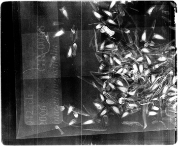
1:5 Magnification
At a 1:5 magnification the clearest results are returned. Each achene can easily be counted, identified as hollow or full, and the label is clearly legible. This magnification is the highest magnification possible on this x-ray machine and is therefore the high-end extreme. The negative aspects of this magnification are that it is not possible to capture the entire envelope in the image. Unless all of the achenes are pushed towards the label there is no way of telling how many achenes may not be accounted for. As a result of not being able to fit one full envelop in the image it is not a far stretch of the mind to understand that capturing two envelopes at this magnification setting is out of the question and that only one envelope (or part of one). At this magnification, it would only be recommend to be used to examine certain achenes in order to inspect damage, shape, or any other anomaly that is being investigated.
Conclusion:
Considering all of the magnification settings, the top two would have to be 1:2 and 1:3. These levels have the most benefits out of all of the other settings without all of the negatives of the other settings. These two options are thus recommend for use. The question that presents itself is a matter of time and efficiency, and what setting is best to use. At the 1:2 setting, does the time saved by scanning two envelopes at a time out weigh the time it would take a person to zoom in on each envelope and count the achenes and determine which are germinated and which are not? At a 1:3 magnification, does the time to scan one envelope at a time and continually switch out samples negate the time it takes for a person to count the germinated and not germinated seeds without zooming in?
After carefully considering the question of time and efficiency I conclude that the 1:2 magnification setting is indeed the best choice and the 1:3 setting the second best choice. The time it takes zoom in on one envelope to count the achenes and determine their germination states and then zoom out and zoom in to do the process over is shorter that the time it takes to scan one envelope at a time and be easily to count the achenes and determine the germination states without needing to zoom in. To zoom in and out and back in takes far less time than completely going through the image scanning process for individual envelopes. The time it takes for the media plate to go through the CR reader is what takes the longest and makes the 1:3 magnification the second best choice.
All accounted for, the best magnification setting to use is 1:2 for time and efficiency sake. If time is not of the essence, then the 1:3 magnification setting would be the best option. The final ranking of all of the magnification settings would be: A.) 1:2 B.) 1:3 C.) 1:4 D.) 1:5 E.) 1:1.5 and F.) 1:1 respectively. This ranking and the best option may very based on the experiment being run, sample size, and what the object of inquiry is. For a general scanning to most efficiently count and determine germination states this ranking holds. If a different experiment is being conducted and or a different sample size or object of inquiry is at hand then the best setting to use should be determined as needed based on the pros and cons as listed in the previous pages.
Howdy folks! This week field work was delayed by a couple of wet spells, but thanks to reinforcements (thanks Ruth!), we conquered seedling refinds at Loeffler’s Corner on Tuesday; East Riley and Riley on Thursday. Due to lack of time/manpower, we decided to scale back on seedling refinds (by focusing on searching circles that were reported to have at least 1 seedling). The frame maps made using R and the frame coordinates we recorded in June were really helpful.
Yesterday after lunch, the 4 of us (Stuart, Josh, Katherine and I) went out to Hegg Lake. I brought my bike out so I could pull in my Dichanthelium flags from my sites at Hegg Lake, and then I biked to C2 to join in the head harvest. I believe we harvested just over half the heads from C2. After that we headed back to Hjelm House and started harvesting in C1 until it was time to go.
This morning we went out to Staffanson in the truck. Stuart, Josh, and Katherine flagged plants for seedling refinds and harvested Echinacea heads as part of Amber Z’s project. I did my final round of collection at Staffanson and then pulled in flags from the plot that was planted with seedlings in June. After lunch, we paired up and continued harvesting in C1. We filled up NINE grocery bags with Echinacea heads in just one afternoon! Uff da! That was really a heck of a harvest! Good job Team Echinacea!
Heya! Here’s Maria reporting from the Town Hall.
Many of our team members had returned to school/civilization in the past 2 weeks: Nicholas, Lee, Amber Z, Amber E, Gretel, Per, Hattie, and Stuart. Thanks to Northwestern’s quarter system, Katherine, Josh and I are still here. I’ll be leaving next Saturday, Katherine the week after, and Josh two weeks later.
For the past week, we’ve been continuing to work in the field while Stuart was at the Chicago Botanic Garden. Here’s a brief recap of what we did:
Monday: Katherine did C1 Phenology & started harvesting while Josh and I finished GPSing flowering Echinacea at Krusemark (after getting stuck with the truck, the GPS went dead on us – Friday was definitely not our lucky day). We joined Katherine and did harvesting for the rest of the day.
Tuesday: Harvesting at Hegg Lake C2 garden & my last round of Dichanthelium harvesting on the way in to C2 and at Loeffler’s Corner. After lunch, we started flagging plants for Seedling Refinds at East Elk Lake Road, and then got started on a few plants.
Wednesday: Katherine worked on C1 Phenology and her aphid experiment, while Josh and I went out to GPS and harvest Dichanthelium at Loeffler’s Corner, Hegg Lake, and Staffanson. We finished GPSing all Dichanthelium sites! After lunch, we continued seedling refinds at EELR.
Thursday: While waiting for the field to dry up, Josh went out to GPS the Astragalus planted in the C1 ditch and his grasses plot. Katherine and I worked on indoors stuff and our own projects. After that we went to EELR and finished seedling refinds for all but 2 plants that would require extra information (like missing maps). After lunch, we did seedling refinds at East of Town Hall.
Friday: Aphid survey and C1 harvesting took us the whole day. Conference call with Stuart at lunch. Josh discovered grapefruit sprouting from seeds in his grapefruit at lunch. Corn-on-the-cobs and lovely eggplants made our day. Big thank you to Bob Mahoney & Dwight & Jean 🙂
The weather is cooling up so we’ll be starting work at 8.30am again. Stuart will be back on the field tomorrow. Hope we’ll have another honest week’s worth of work! 😀
|
|