|
|
Hi Flog following!
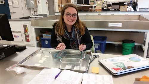
I’m excited to have worked in the Echinacea Project’s lab at the Chicago Botanic Garden for the past few days. While I was here, I worked on the seed set portion of my summer 2017 REU project (which I have now named Barto’s Nice Experiment), and I caught up with many friends from the field season. It’s definitely been a fun week for me in the Chicago area!
At the end of the summer, the team collected my experimental Echinacea heads from the Nice Island remnant in Minnesota after I left. When I came to the garden with Tracie on Thursday of last week, I began dissecting them. I started by separating all rows from each other, but I quickly realized I was only able to accurately distinguish the odd rows (which had painted bracts). To work efficiently, I categorized all achenes into 4 groups based on where they came from in each head: Row 1, Row 3, Row 5, Row 7, or Even Row. Between Thursday, Friday, and the first half of today, I cleaned my 21 experimental heads. Each of the odd rows were put into their own baggie and attached to an x-raying sheet. With the guidance of Tracie, I was able to capture images that show the fullness of all of my odd-row achenes. With this data, I can create a GLM in R like I did with my pollination data from the summer and model which experimental variables (row within the capitulum, style age, and pulse/steady pollination treatment) affected the seed set in my experiment.
For now, I am going to count the full/partially full/empty achenes in my x-rays and get ready to return to Arkansas tomorrow.
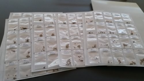
 Ashley working in the Echinacea Project lab at the Chicago Botanic Garden. Setting up the achenes for x-raying! Each of the baggies here has one row’s worth of achenes.  Final x-ray product for one row of achenes.
Hello, Nina here! These past few months, I was an extern with the Echinacea project, looking specifically at data collected last summer about Echinacea success and surrounding plant diversity. My findings are summarized in the report that I’ve attached here.
Trevor Hughes
Prof. Wagenius
8 December 2017
Field Site Burning Effects on Liatris and Solidago Species: Year 2
Background Info:
Habitat fragmentation threatens the livelihood of many remnant prairie populations in the midwestern United States. This is the result of various biological mechanisms such as limited genetic diversity and transformation of the surrounding ecosystem, both of which yield direct effects on the plant species coexisting there (Newman and Pilson 1997, Saccheri et al. 1998). Through either modification potential mates location as well as other changes in pollinator behavior, the reproduction of these species is left especially vulnerable to change (Wagenius 2006). These reproduction patterns are measured in what is commonly referred to as seedset, or the percentage of fertile achenes (those that possess an embryo) out of a certain grouping of total achenes; therefore, seedset effectively displays the relative amount of achenes that are fertile on any given inflorescence.
Previous research reveals that both pollinator activity and respective reproduction of native plant species decrease with habitat fragmentation; as well, many of these studies focused on select species, namely the Echinacea angustifolia, a common plant species often found in midwestern prairie remnant habitats (Wagenius 2006). Differing from prior research, this study focuses on how a contemporary trend—the burning of a specific remnant prairie habitat—could be affecting the reproductive activity of remnant prairie plant species. Expanding beyond Echinacea, this study focuses on two other key prairie species: Liatris and Solidago. By examining two different sides (east and west) of a specific remnant prairie site where the east and west sides are burned interchangeably on a repeating pattern: east side burned, west side burned, and no side is burned. This report analyzes the findings concerning the second year of the study, where no field site was burned. While the specific findings discussed will be limited to this year’s data, with next years data, the study hopes to aggregate all years to yield some conclusions as to the effects of field site burning on reproduction of prairie plant species. Aside from investigating the possible effect that field-site burning has on the seedset of the plant species in the area, it also hopes to be able to provide comparable findings between Liatris, Solidago, and Echinacea so that findings regarding habitat fragmentation can be generalized to more prairie plant species in the future.
Methods:
Liatris and Solidago were gathered at the Staffanson site within the Douglas county in western Minnesota (centered near 45°49’ N, 95°43’ W). They were collected using a randomized method, with 90 Liatris and 74 Solidago inflorescences collected in total. However, the Liatris and Solidago species were collected from both the East and West sides of the Staffanson site, but a blind-procedure was used to ensure this was not known during the data collection or analysis process. It should be noted that while the West field site was burned last year, no field site was burned this year in preparation for burning the East field site and continuing the cycle in 2018.
Following the collection process, the Liatris and Solidago inflorescences were randomized using excel software and put in their appropriate order, divided by species. This prevents bias at multiple steps during the course of data collection, including cleaning, counting, and x-raying. Beginning with Liatris, a bag was selected according to the random order and all heads were removed from the inflorescence to be cleaned. Next, thirty achenes were selected randomly using a grid system under the container to be used as an x-ray sample for that inflorescence. The remaining achenes were separated from any chaff and placed in an envelope for future reference and potential research. This process was repeated with all 90 Liatris samples. Additionally, beginning with the 50th randomized Liatris sample and continuing until all remaining Liatris samples were cleaned, the number of achenes in the top, middle, and bottom head were also recorded in a spreadsheet. If there was no clear middle, the achene closest to the bottom relative to the midpoint was chosen.
The Solidago process was quite similar. The bags were selected in a pre-randomized order and the inflorescence was removed to be cleaned. However, due to the considerable number of achenes on most Solidago inflorescence, it would be impractical to attempt to use all achenes for cleaning; therefore, I simply shook each inflorescence for 10 seconds and used those achenes for further analysis. From there, 30 achenes were randomly placed into a small plastic baggie for x-raying whilst other achenes were separated and placed into an envelope for further comparison. This process was repeated for all 74 solidago samples.
After the cleaning was completed, the baggies were placed on sheets to prepare for x-raying. Twenty samples were x-rayed at a time and there scans were recorded. Lastly, the x-ray samples were counted for the number the number of achenes in each sample that actually contained a fertile embryo; in this way, the seed-set of the Liatris and Solidago achenes was recorded so that comparisons between the east and west Staffanson field sites could be made.
Results:
All data was aggregated and analyzed with use of various statistical tests on the R platform; all figures and/or tables were also made on this same platform. Data regarding the top/middle/bottom breakdown of Liatris along with the seedset of Liatris and Solidago on the east and west sides of the Staffanson site were analyzed for potential findings.
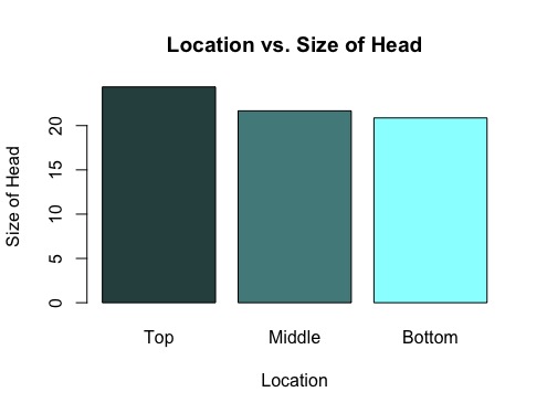
Figure 1: Location of Head vs. Size of Head in Tops/Middles/Bottoms of Liatris

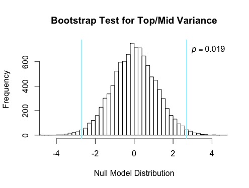
The tops of the Liatris species were found to have the greatest number of achenes with a mean number of achenes of 24.367, middles followed with a mean of 21.667, and bottoms yielded the lowest mean at 20.867 (see Figure 1). A bootstrap test was conducted between the means of the tops and middles, generating a p-value of 0.019, meaning that there is only a 1.9% chance that the difference in size of head betweenst tops and middles would be found by chance simply by sampling randomly from inflorescences (see Figure 2). While a p-value was not calculated for the difference in size of head amongst tops and bottoms, it is speculated that this analysis would yield a even lower p-value than tops and middles due to the greater difference in mean. While a bootstrap test was run between middles and bottoms, this yielded a high p-value and indicated there was a large possibility that the difference between middles and bottoms of Liaris could be found by chance from sampling randomly and was therefore not determined to be an meaningful finding.
Figure 2: Bootstrap Test for variance between Tops and Middles of Liatris
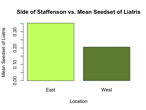
The data collected on seedset for the 90 Liatris samples was aggregated and eventually divided between East and West lines of the Staffanson site. The mean seedset was calculated for each side and are compared below (see Figure 3). The East meen seedset of Liatris was 35.2%, which towers over the West’s 20.6%.
Figure 3: Side of Staffanson Site vs. Mean Seedset of Liatris
A bootstrap test was run on this dichotomy to determine the confidence intervals of these findings as well as the p-value. The ablines were found to fall outside of the normal distribution, yielding a p-value of 0.1%, indicating that this difference has a very little possibility of resulting from chance and that the difference in seedset between the East and West is quite noteworthy and telling of other possible differences between these two sites. The confidence intervals were not found to overlap, strengthening the certainty of my findings (see Figure 4).
Figure 4: East and West Sides of Staffanson vs. Mean Seedset of Liatris with 95% C.I.
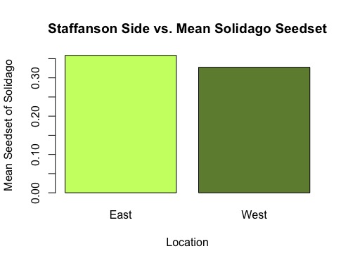
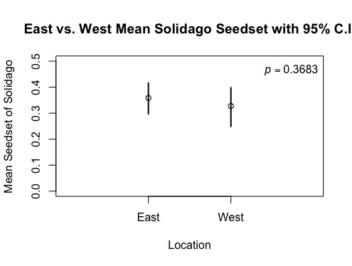
Identical tests were conducted on the 74 Solidago samples and respective seedset data, but different findings were discovered. The seed-set data collected for Solidago was divided between the east and west sides of the Staffanson site. The mean seed-sets of each side were calculated, revealing to be 35.9% for the east and 32.7% for the west (see Figure 5). This demonstrates that the east had a higher seed-set, but not at the same large interval seen with the Liatris species. Confidence intervals and a p-value were also determined for each side. The p-value was revealed to be 36.45%, which indicates the potential for this difference in seed-set to result a large portion of the time from natural variation, and not possibly due to the difference in side of the Staffanson site (see Figure 6). Supporting this large p-value, the confidence intervals also overlap, indicating that the variables could potentially swap and vary greatly in repeating this study, generating further doubt on the implications of this finding.
Figure 5: Side of Staffanson Site vs. Mean Seedset of Solidago
Figure 6: East and West Sides of Staffanson vs. Mean Seedset of Solidago with 95% C.I.
Discussion:
Firstly, the data regarding the tops/middles/bottoms of Liatris demonstrate a definite correlation among location and size of head. Based on the low p-value, it can be determined that the tops have the greatest number of achenes, compared to the middles and bottoms, but whether or not there is a significant difference in the number of achenes betweenst middles and bottoms cannot be directly determined from this data set. While this data indicates a trend between location and size of head (with greatest numbers of achenes found among the top heads), more samples should be collected and analyzed to strengthen this finding, specifically with regards to the difference in size between middles and bottoms.
Before the data from this years seedset among the east and west sides of the Staffanson site can be analyzed, the findings from last year’s study (when the West side was burned), must be discussed. The 2016 data indicates that the West had a higher mean seedset than the East for Liatris, but there was little to no correlation between the east and west with Solidago. This finding is interesting for a couple of reasons. For one, this directly contrasts with my data from this year (where no sides were burned), as now the east had nearly a 75% increase in seedset compared to the West. Interestingly, the east side now has the larger seedset, meaning the sides of the field swapped by a large margin. This also contrasts with what one would expect with a field burning, which generally is speculated to stimulate growth, achene development, and seedset. However, it appears from this data set that the burning possibly hinders achene development and seedset, but this cannot be completely determined from this data set. The data from 2018 (when the East side is burned), would be vital for drawing this conclusion.
Interestingly enough, while the data sets contradict themselves on these grounds, they agree on one important point: field site burnings have a greater impact on Liatris than Solidago. This raises questions as to what biological mechanism within each species accounts for this difference. Once again, data from 2018 would also be vital for making a definitive conclusion as to why field site burning seems to have a lessened impact on the Solidago species.
 Anna and Will decapitate a plant. It’s Echinacea pallida which is not native to Minnesota. Echinacea pallida is an Echinacea species that is not native to Minnesota. In July 2017, we identified 100 flowering E. pallida plants with 222 heads that were planted in a restoration at Hegg Lake WMA. Every year for the past several years, we have visited the E. pallida plants, taken phenology data, and chopped off their heads. On July 7, 2017 when we collected the data, the maximum male row was 19, meaning flowering started about 19 days earlier–June 18, 2017. E. angustifolia in the remnants started flowering on June 24, about a week later. 17 of the 222 E. pallida heads were still buds on 7 July, so these plants would have continued flowering for awhile.
We went back to check if we missed any heads on 31 August and found two. They were done flowering, but hadn’t dropped seeds.
Start year: 2011
Location: Hegg Lake WMA restoration
Overlaps with: Echinacea hybrids (exPt6, exPt7, exPt9), flowering phenology in remnants
Physical specimens: 222 heads were cut from E. pallida plants and likely decomposed. We brought two heads back with us to Chicago.
Data collected: A csv in ~Dropbox/remData/105_assessPhenology/phenology2017 with tag, row number the male florets were at on July 7, 2017 for each head, and initials of the data collector.
GPS points shot: We shot points for the 100 flowering E. pallida plants.
Products: In Fall 2013, Aaron and Grace, externs from Carleton College, investigated hybridization potential by analyzing the phenology and seed set of Echinacea pallida and neighboring Echinacea angustifolia that Dayvis collected in summer 2013. They wrote a report of their study.
Previous team members who have worked on this project include: Nicholas Goldsmith (2011), Shona Sanford-Long (2012), Dayvis Blasini (2013), and Cam Shorb (2014)
You can find more information about Echinacea pallida flowering phenology and links to previous flog posts regarding this experiment at the background page for the experiment.
 Marisol, our 2017 Lake Forest College intern! This fall the Echinacea Project had a Lake Forest College intern, Marisol. In Marisol’s 16-hour internship over 4 weeks, she accomplished a lot! Her primary goal was to assess if the seed counter will be useful in our ACE protocol. Currently, volunteers scan achenes and then count them with our counting software online. The seed counter could potentially remove these steps and make the process more efficient.
Marisol did a few experiments with the seed counter. She determined the best sensitivity and speed settings for counting Echinacea achenes, by running packs of achenes through the seed counter multiple times and comparing those counts to her manual counts. She found that the most accurate sensitivity and speed is 8 and 70, respectively.
Marisol also determined the types of achenes that get counted and the types of achenes that often get missed. Usually, achenes that are really small, thin, and broken don’t get counted at all. Broken achenes that are still pretty large often get counted (about 2/3 of the time). Achenes that are full and above a certain size get counted 100% of the time.
In the mini-internship class, Marisol presented her findings to her classmates. See her poster below!
 Marisol’s final poster for her mini-internship! Click to enlarge.
This year, the number of flowering plants in our main experimental plot (exPt1) dropped in half compared to last year. This might be due to the lack of a burn in the prior fall or spring. Plot 2 (exPt2) had about the same number of heads in ’16 & ’17.
In exPt1, we kept track of approximately 72 heads. The peak date was July 19th. The first head started flowering on July 2nd and the last head finished up on August 21st. In contrast, we kept track of 1076 heads in exPt2, about 140 more than last year! The peak date for these Echinacea was a bit earlier, July 13th. exPt2 heads also started and ended earlier (June 22 – August 19).
We harvested the heads at the end of the field season and brought them back to the lab, where we will count fruits (achenes) and assess seed set.
 Flowering schedules for 2017 in exPt1 and exPt2. Black dots indicate the number of flowering heads on each date. Gray horizontal line segments represent the duration of each head’s flowering and are ordered by start date. The solid vertical line indicates peak flowering, while the dashed lines indicate the dates when 25% and 75% of heads had begun flowering, respectively. Note the difference in y-axes between the two plots. Click to enlarge! Start year: 2005
Location: Experimental Plots 1 and 2
Overlaps with: Heritability of flowering time, common garden experiment, phenology in the remnants
Physical specimens: Harvested heads from both experimental plots are in the lab at CBG. The ACE protocol for these heads will begin soon.
Data collected: We visit all plants with flowering heads every 2-3 days starting before they flower until they are done flowering to record start and end dates of flowering for all heads. We managed phenology data in R and added it to our long-term dataset. The figures above were generated using package mateable in R. If you want to make figures like this one, download package mateable from CRAN!
You can find more information about phenology in experimental plots and links to previous flog posts regarding this experiment at the background page for the experiment.
Nina here! Today was Trevor and I’s last day of our externship, which was bittersweet. Although I’m very excited to sleep in past 6:30, I’m definitely going to miss our mentors, Tracy, Lea, and Stuart, as well as all of the volunteers and the whole Botanic Garden community that we briefly got to know during our time here. Trevor and I mostly continued working on our papers, but we also gave short presentations of our projects to the lab to practice presenting. We also had closing interviews regarding our experiences and our thoughts on the externship. Trevor and I have both really enjoyed our time with the Echinacea project, and we hope that you will stay tuned for our final papers, which will be coming very soon (either this weekend or on Monday).

Thanks for everything,
Nina 🙂
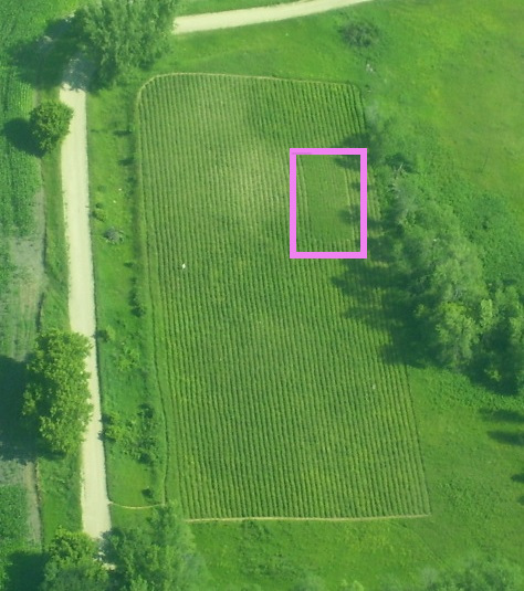
 exPt 1 showing the main planting of the 1999 cohort outlined in purple In 2017 only 11 plants flowered of the surviving 750 plants in the 1999 cohort. That means that 57% of the original 1,303 plants are surviving and only 1.5% of the living individuals flowered! 2.4% of living individuals flowered in 2016. In contrast, 29% of living plants flowered in 2015. We are not sure why so few plants flowered this year. It’s possible that lack of fire in the plot influenced flowering rates. This plot was due for a prescribed burn in spring 2017, but weather and scheduling conflicts kept us from burning.
Stuart described the provenance of the 1999 cohort, “The 99 cohort came from the seeds of plants that flowered in 1998 that we used to estimate seed set.” The cohort was divided into a planting in the main exPt1 and a planting in a plot south of there, near the farmhouse. These plants are part of a common garden experiment designed to study differences in fitness and life history characteristics among remnant populations. Every year, members of Team Echinacea assess survival and measure plant growth and fitness traits including plant status (i.e. if it is flowering or basal), plant height, leaf count, and number of flowering heads. We harvest all flowering heads in the fall, count all achenes, and estimate seed set for each head in the lab.
Start year: 1999
Location: Experimental plot 1
Overlaps with: phenology in experimental plots, qGen3
Physical specimens:
- Although 11 plants flowered, only 4 normal heads were harvested from the 1999 cohort. At present, they await processing in the lab to find their achene count and seed set.
Data collected:
- We used Visors to collect plant growth and fitness traits—plant status, height, leaf count, number of flowering heads, presence of insects—these data have been added to the database
- We used Visors to collect flowering phenology data—start and end date of flowering for all individual heads—which is ready to be added to the exPt1 phenology dataset
- Eventually, we will have achene count and seed set data for all flowering plants (stay tuned)
Products:
Trevor here! And for, sadly, what is the last time. I can’t believe time flew by so fast! Alas, Nina and I began writing our research papers as we near the end of our externship experience. Our “mini-papers” will be available on the flog and our broken down into four sections: introduction, methodology, results, and discussion. Make sure to check them out! Nina’s will be about diversity of plant species and its affect on Echinacea seed-set, while mine will concern how the burning of certain sides of a field-site affect the seed-set Liatris and Solidago species. Nina and I also had our “dissertation defense” sessions with Stuart, which both were very enjoyable and left us with lots of answers, but also plenty of questions to consider as we move forward as both students and researchers.

We also got to attend Dr. Kelly Ksiazek Mikenas public dissertation defense discussing her research on green roofs in both Chicago and Germany. In fact, the green roof pictured above is quite famous and is located on top of Chicago’s very own City Hall! Her talk was extremely enlightening and taught me a lot about promoting biodiversity in an urban setting. She defended the use of prairie species on green roofs in cities. She also had a wonderful array of snacks and her resume was quite inspiring and left me lots to think about when it comes to my future.
Thanks for everything Team Echinacea,
Trevor
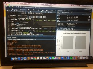
Nina here! Today, Trevor and I continued analyzing the data that we collected during the first two weeks of our externship. We both kept working in R, perfecting our papers, and analyzing our results.
Trevor found the confidence intervals for mean seed-set for Liatris and was very excited to see that the two intervals didn’t overlap, strengthening his confidence in his previous findings. Next, he aggregated and merged Solidago data before repeating the analysis he did for Liatris on the Solidago data, but with very different results. It seems as if Solidago was not effected by the burn that occurred in the site (as you can see from the photo on the left), but stay tuned for more updates!

Meanwhile, I looked the diversity function within R’s ‘vegan’ package to use Shannon’s and Simpson’s Diversity Indices on my plant community from each plot. I plotted seed-set, fecundity, and achene count against each index and found the highest correlation when looking at achene count. Next, I calculated species richness as well as the Shannon’s and Simpson’s Diversity Indices including only flowering plants. More updates to follow! After finishing up my actual analysis, I got back to working on my paper (which you can see a preview of on the right) and started thinking about which portions of my results and which graphs I might want to include in my paper.
|
|