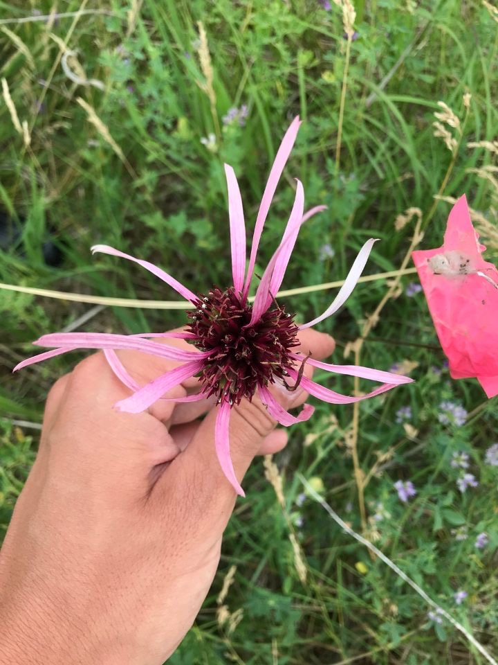
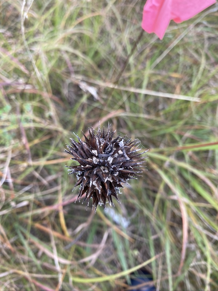
Echinacea pallida flowering phenology:Echinacea pallida is a species of Echinacea that is not native to Minnesota. It was mistakenly introduced to our study area during a restoration of Hegg Lake WMA. Since 2011, Team Echinacea has visited the pallida restoration, taken flowering phenology, and collected demography on the non-native. We have decapitated all flowering E. pallida each year to avoid cross-pollination with the local Echinacea angustifolia. Each year, we record the number of heads on each plant and the number of rosettes. We also get precise gps coordinates of all plants and then chop the flowering heads off! This year, we cut E. pallida heads off on July 6th and 8th. We shot gps points as they were found; in the fall, we revisited the plants and did not find any stragglers.
Overall, we found and shot 143 flowering E. pallida plants, and 433 heads in total, averaging 3.02 heads per plant. The average rosette count was 5, the maximum was 27 rosettes — absolutely massive!! When recording data on E. pallida, we forgot that we needed phenology data, so the data from the 6th does not have any phen at all, and the data from the 8th is in the demo form in notes as a string. We do not have very accurate data on phenology of E. pallida this year, but our estimated first day flowering is June 22nd.
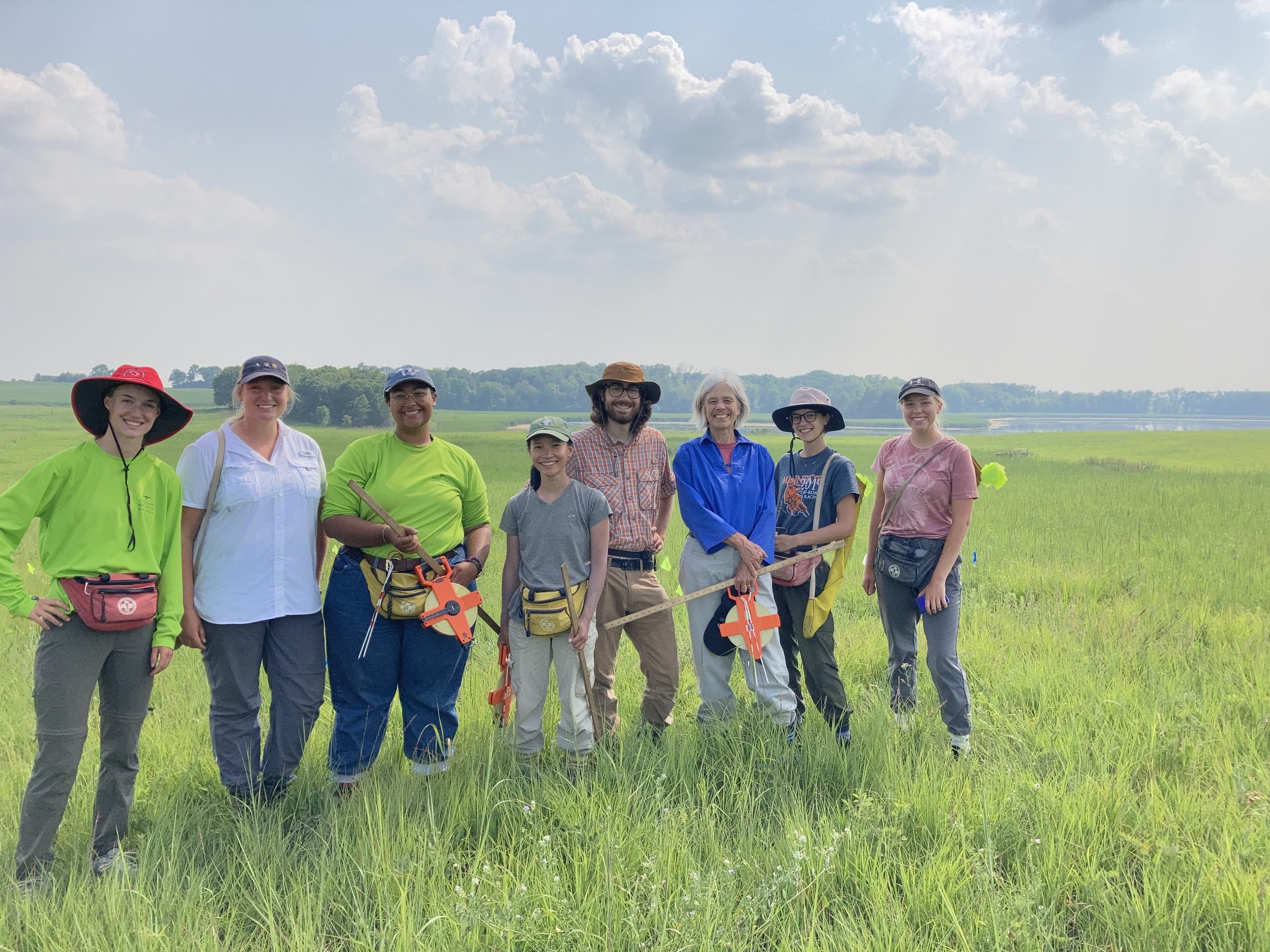
Pallida demo/cut/surv involved 7 different people working a total of 1170 minutes (19.5 hours) on 3 separate days.
Location: Hegg Lake WMA Start year: 2011
You can find more information about E. pallida flowering phenology and previous flog posts on the background page for the experiment.
exPt6: Experimental plot 6 was the first E. angustifolia x E. pallida hybrid plot planted by Team Echinacea. A total of 66 Echinacea hybrids were originally planted; all have E. angustifolia dams and E. pallida sires. In 2021, we visited 31 positions and found 15 living plants. No plants have flowered in this plot yet.
Location: near exPt8 Start year: Crossing in 2011, planting in 2012
You can find more information about experimental plot 6 and previous flog posts about it on the background page for the experiment.
exPt7: Planted in 2013, experimental plot #7 was the second E. pallida x E. angustifolia plot. It contains conspecific crosses of each species as well as reciprocal hybrids. There were 294 plants planted. This summer, we visited 176, and of these plants, only 136 plants were still alive. There were 13 flowering plants this year! This is the most flowering plants that this plot has produced. These 26 flowering plants produced 26 heads. We have not yet used the pedigree data to see what number of these plants are hybrids or not.
Location: Hegg Lake WMA Start year: Crossing in 2012, planting in 2013
You can find more information about experimental plot 7 and previous flog posts about it on the background page for the experiment.
exPt9: Experimental plot 9 is a hybrid plot, but, unlike the other two hybrid plots, we do not have a perfect pedigree of the plants. That is because the E. angustifolia and E. pallida maternal plants used to generate seedlings for exPt9 were open-pollinated. We need to do paternity analysis to find the true hybrid nature of these crosses (assuming there are any hybrids). There were originally 745 seedlings planted in exPt9. We found 261 living plants in 2021, 20 of which were flowering, with 42 heads! There were 138 plants that we searched for but could not find.
Location: Hegg Lake WMA Start year: 2014
You can find out more information about experimental plot 9 and flog posts mentioning the experiment on the background page for the experiment.
Measuring p6/7/9 involved 8 different people working a total of 1380 minutes (23 hours) on 2 separate days.
Experimental plots 6, 7, and 9 all burned this year. The peak in number of flowering plants in both p7 and p9 this year is indicative of the effect fire can have on flowering in Echinacea. In the past we have bagged heads in these plots but this year we did not.
Data collected for exp679: For all three plots, we collected rosette number, length of all leaves, and herbivory for each plant. We used visors to collect data electronically, and it is still being processed to be put into our SQL database.
Data collected for E. pallida demography and phenology: Demography data, head counts, rosette counts, gps points shot for each E. pallida. Find demo and phenology visor records in the aiisummer2021 repository. GPS coordinates can be found in demap. As mentioned above, all phenology data from July 8th can be found in demo. For more details, see aiiSummer2021/demo/pallidaPhen.R.
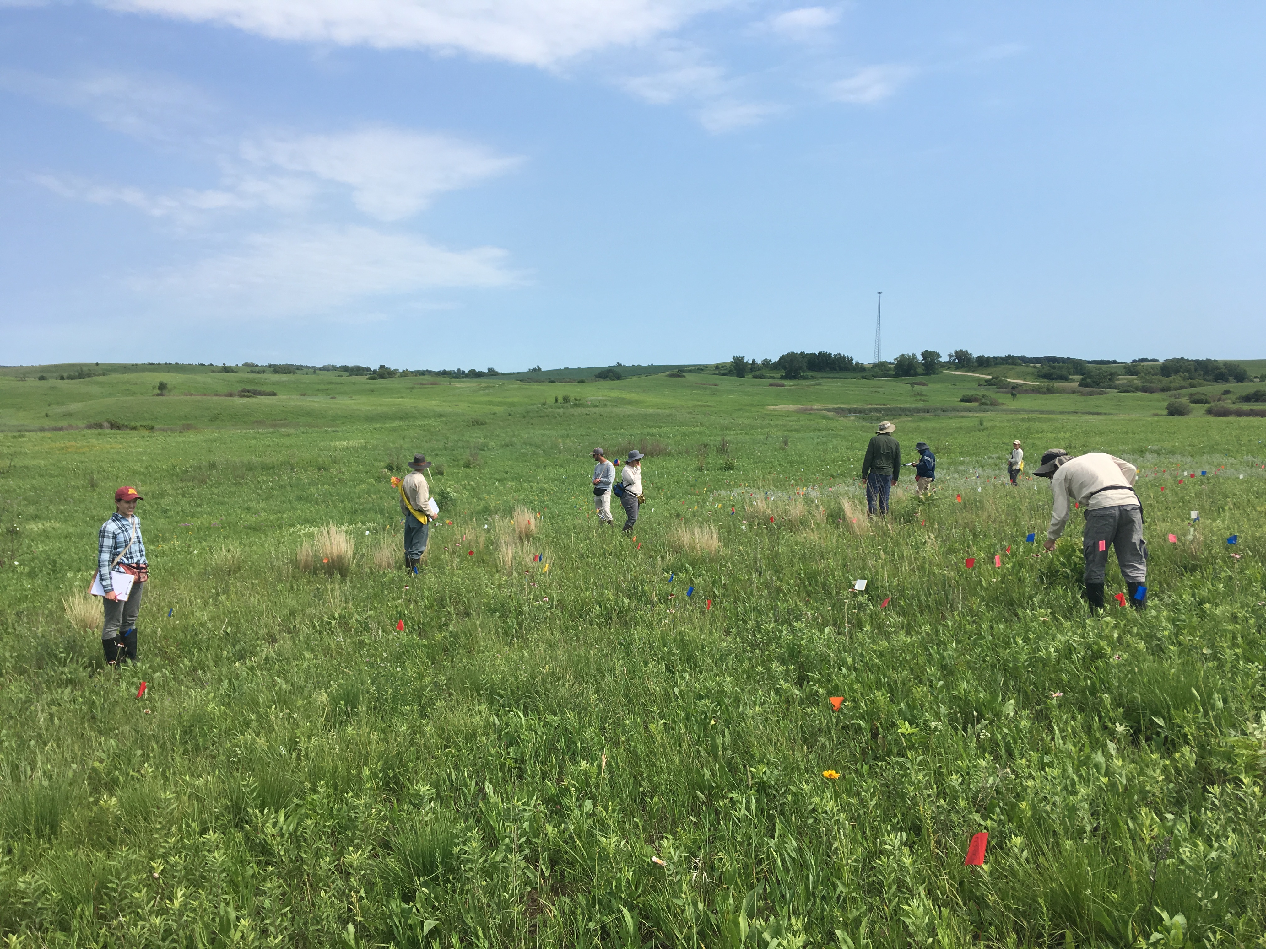
The crew poses after knocking out measuring half of p7 and p9
Echinacea pallida Flowering phenology:Echinacea pallida is a species of Echinacea that is not native to Minnesota. It was mistakenly introduced to our study area during a restoration of Hegg Lake WMA. Since 2011, Team Echinacea has visited the pallida restoration and taken flowering phenology and collected demography on the non-native. We have decapitated all flowering Echinacea pallida each year to avoid pollination with the local Echinacea angustifolia. Each year we record the number of heads on each plant and the number of rosettes. We also get precise gps coordinates of all plants and then chop the flowering heads off! This year we cut E. pallida heads off on June 30th. We revisited plants and shot gps pointson September 17th 2020. When shooting points, we found two E. pallida plants that had missed the big decapitation event. We harvested the heads before any fruit dispersed.
Overall, we found and shot 99 flowering E. pallida. On average, each plant produced 1.96 flowering heads, with a total of 194 beheadings. The average rosette count was 6.1, the maximum was 31 rosettes — absolutely massive!!
Location: Hegg Lake WMA Start year: 2011
exPt6: Experimental plot 6 was the first E. angustifolia x E. pallida hybrid plot planted by Team Echinacea. A total of 66 Echinacea hybrids were originally planted; all have E. angustifolia dams and E. pallida sires. In 2020, we visited 40 positions and found 22 living plants. No plants have flowered in this plot yet. Location: near exPt8 Year started: Crossing in 2011, planting in 2012
You can find more information about experimental plot 6 and previous flog posts about it on the background page for the experiment.
exPt7: Planted in 2013, experimental plot # 7 was the second E. pallida x E. angustifolia plot. It contains conspecific crosses of each species as well as reciprocal hybrids. There were 294 plants planted, of these plants only 148 plants were still alive. There were 2 flowering plants this year! One was the progeny of a E. pallida x E pallida cross and the other of these flowering plants was a hybrid of E. pallida X E. angustifolia! This is the first hybrid to bloom. Anna M. investigated the compatibility of this hybrid with E. pallida and E. angustifolia by performing a series of hand crosses.
Location: Hegg Lake WMA Start year: Crossing in 2012, planting in 2013
exPt9: Experimental plot 9 is a hybrid plot, but, unlike the other two hybrid plots, we do not have a perfect pedigree of the plants. That is because E. angustifolia and E. pallida maternal plants used to generate seedlings for exPt9 were open-pollinated. We need to do paternity analysis to find the true hybrid nature of these crosses (assuming there are any hybrids). There were originally 745 seedlings planted in exPt9. We found 391 living plants in 2020, three of which were flowering! Two of these plants were technically “flowering” because they produced buds, but they produced zero flowering heads because no flowers ever opened (no pollen or fruits). There were 105 plants that we searched for but could not find. Location: Hegg Lake WMA Start year: 2014
You can find out more information about experimental plot 9 and flog posts mentioning the experiment on the background page for the experiment.
There were a total of three flowering heads between the three plots, we collected flowering phenology data on these heads. Flowering started on June 28th and ended between July 7th and 23rd. There were two additional flowering plants that only produced duds.
Data collected for exp679: For all three plots we collected rosette number, length of all leaves, and herbivory for each plant. We used visors to collect data electronically and it is still being processed to be put into our SQL database.
Data collected for E. pallida demography and phenology: Demography data, head counts, rosette counts, gps points shot for each E. pallida. Find demo and phenology visor records in the aiisummer2020 repository. GPS coordinates can be found in demap.
Look at this three-headed E. pallida monster we found! Shown at the beginning and end of season
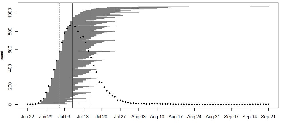
In 2020, we collected data on the timing of flowering for 855 flowering plants (1071 flowering heads) in 31 remnant populations. The plants ranged from having 1 to 8 flowering heads. The earliest bloomers initiated flowering on June 22nd . Plant 22195 at NWLF was the latest bloomer, only beginning to shed pollen on September 14th, nearly a month after the second-latest flowering plant had ceased producing pollen (August 18th). As is typical for the latest bloomer of a season, township mowers had mowed over this plant earlier in the season, which is perhaps why it took longer for it to sprout a new flowering stem. Peak flowering was on July 9th, when 886 heads were flowering.
A major part of the motivation behind this year’s effort in monitoring phenology was to collect baseline data on flowering rates and timing. Team Echinacea recently received funding to perform prescribed burns in these populations. Next summer, we will compare flowering patterns in populations before and after fires to understand how burns drive the effects of timing of flowering on mating patterns and fitness of individuals in natural populations.
Start year: 1996
Location: Roadsides, railroad rights of way, and nature preserves in and around Solem Township, MN
Overlaps with: phenology in experimental plots, demography in the remnants, gene flow in remnants, reproductive fitness in remnants
Data/materials collected: We identify each plant with a numbered tag affixed to the base and give each head a colored twist tie, so that each head has a unique tag/twist-tie combination, or “head ID”, under which we store all phenology data.We monitor the flowering status of all flowering plants in the remnants, visiting at least once every three days (usually every two days) until all heads were done flowering to obtain start and end dates of flowering. We managed the data in the R project ‘aiisummer2020′ and will add the records to the database of previous years’ remnant phenology records, which is located here: https://echinaceaproject.org/datasets/remnant-phen/. The dataset is ready to be updated, but I don’t believe it has been at the time of writing.
A flowering schedule for individuals from all remnants. Notice the gap between when second-to-last flower ceased pollen production and when the latest bloomer began on September 14th!
A flowering curve (created here using the R package mateable) summarizes the flowering phenology data that we collected in 2020, indicating the number of individuals flowering on a given day and the flowering period for all individuals over the course of the season.
We shot GPS points at all of the plants we monitored. Soon, we will align the locations of plants this year with previously recorded locations and given a unique identifier (‘AKA’). We will link this year’s phenology and survey records via the headID to AKA table.
You can find more information about phenology in the remnants and links to previous flog posts regarding this experiment at the background page for the experiment.
Products: A dataset of flowering phenology is ready to be posted on the website. It is currently located in Dropbox\remData\105_assessPhenology\phenology2020\phen2020_out and is available upon request. The headIds in this dataset have not yet been merged with the akas (long-term identifiers) in the demography dataset.
In 2019,
we collected data on the timing of flowering for 95 flowering plants (127
flowering heads) in 8 remnant populations, which ranged from 1 to 29 flowering heads.
The earliest bloomers (four plants at four different remnants) initiated
flowering on July 4. Plant 24050 in the aptly named remnant population North of
Northwest of Landfill was the latest bloomer, shedding its last anthers of
pollen on August 16. Township mowers had mowed over this plant earlier in the
season, which is perhaps why it took longer for it to sprout a new flowering
stem. Altogether, the flowering season was 43 days long. Peak flowering was on
July 19, when 105 heads were flowering.
This season
marked the 19th season of collecting phenology records in remnant populations! Though
we do not have data for all populations every year, Stuart monitored phenology
in all of our remnant populations in 1996 and in following years (2007, 2009,
2011-2019) students and interns studied phenology in particular populations. From
2014-2016, determining flowering phenology was a major focus of the summer
fieldwork, with Team Echinacea tracking phenology in all plants in all of our
remnant populations. The motivation behind this study is to understand how
timing of flowering affects the mating patterns and fitness of individuals in
natural populations.
Flowering
occurred much later this season than previous years, with peak flowering
falling a full 14 days later in the year than 2018, when flowering started on
June 20, and 10 days later than 2017. Of all the years that we data for flowering
phenology in the remnant populations in and around Solem Township, this season was
the second-latest, with only the 2013 season beginning later, on July 6.
However, this observation comes with the caveat that sampling effort varied
between years and some years focused on particular contexts, such as population
where a portion had experienced a spring burn (see Fire and Flowering at SPP). Many other plants and animals in
Minnesota seemed to have delayed phenology this spring and summer, perhaps a
result of an unusually wet and snowy spring.
Start
year: 1996
Location: Roadsides,
railroad rights of way, and nature preserves in and around Solem Township, MN
Overlaps
with: phenology in experimental plots, demography in the
remnants, gene flow in remnants, reproductive fitness in remnants
Data/materials
collected:We identify each plant with a numbered tag affixed to
the base and give each head a colored twist tie, so that each head has a unique
tag/twist-tie combination, or “head ID”, under which we store all phenology
data.We monitor the flowering status of all flowering plants in
the remnants, visiting at least once every three days (usually every two days)
until all heads were done flowering to obtain start and end dates of flowering.
We managed the data in the R project ‘aiisummer2019′ and added the records to
the database of previous years’ remnant phenology records, which is located
here: https://echinaceaproject.org/datasets/remnant-phen/.
A flowering curve (created here using the R package mateable) summarizes the flowering phenology data that we collected in 2019, indicating the number of individuals flowering on a given day and the flowering period for all individuals over the course of the season.
We shot
GPS points at all of the plants we monitored. Soon, we will align the locations
of plants this year with previously recorded locations and given a unique
identifier (‘AKA’). We will link this year’s phenology and survey records via
the headID to AKA table.
We
harvested a random sample of 1/3 of the flowering heads from each remnants in
August and September, plus an X additional heads from populations that were highly
isolated, for a total of X harvested seedheads. These are currently stored at
the University of Minnesota. This winter, I will assess the relationship
between phenology and reproductive fitness by x-raying all of the seeds we collected.
In addition, I will determine the paternity (i.e., pollen source) for a sample
of seeds by matching the seed genotype to the potential pollen donors. Doing so
will shed light on how phenology influences pollen movement and gene flow
patterns.
You can
find more information about phenology in the remnants and links to previous
flog posts regarding this experiment at the background
page for the experiment.
Products: I presented a poster based on the
locations and flowering phenology of individuals from summer 2018 at the
International Pollinator Conference in Davis, CA this summer. The poster is
linked here: https://echinaceaproject.org/international-pollinator-conference/.
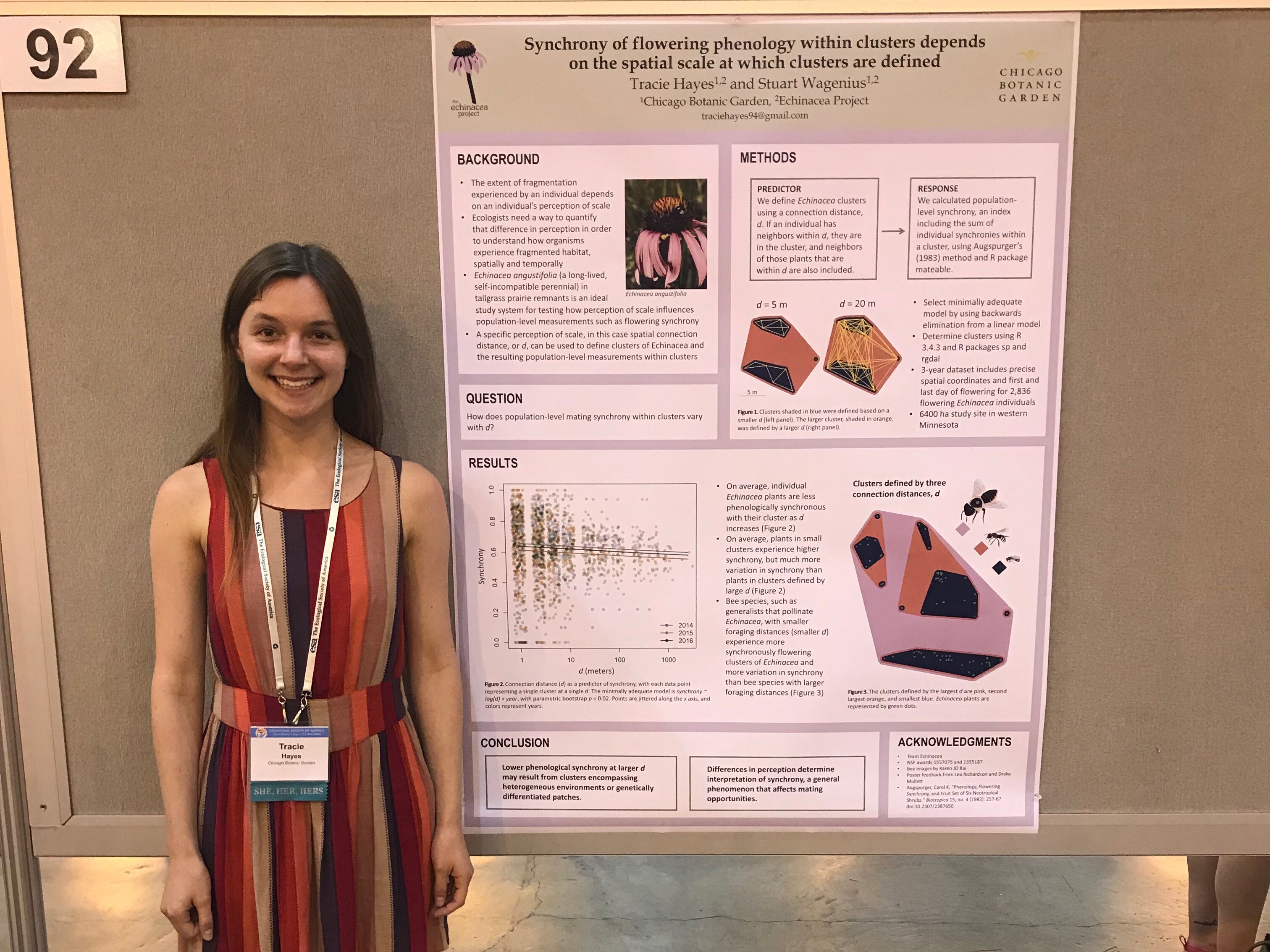
Last week, I attended ESA for the first time and presented a poster on a project I’ve been working on for the past few months: how the synchrony of flowering phenology within clusters of Echinacea depends on the connection distance used to define those clusters. I presented on Tuesday, August 7, 2018 in PS 18: Habitat Structure, Fragmentation, Connectivity from 4:30-6:30, board #92 (just feet away from Will’s poster). My main results are that clusters of Echinacea defined by a small connection distance tend to have lower synchrony on average than clusters defined by larger connection distances. Clusters defined by smaller connection distances also have more variation in synchrony. In terms of a bee’s perspective, this could mean that bees with smaller foraging distances are experiencing more synchronous clusters of Echinacea as they travel from one plant to the next. However, the experience from one small bee to the next is variable. Larger bees with larger foraging distances might be experiencing clusters that are more asynchronous, so as they travel from one Echinacea to the next, plant flowering times might not be overlapping as much.
There was an almost continuous flux of people coming by, and even though I was nervous at first, these couple of hours were probably my favorite part of the conference. Even if some of the listeners didn’t ask me specific questions at the end, just describing my project over and over made me realize what parts I wanted to continue thinking about and working on. I had scientists come by that I recognized from talks I had seen, Team Echinacea alumni interested in what we are doing now, and people I didn’t know that just came because of the title! It was all really exciting and I have a page of notes with questions and ideas to think about as I move forward with this project.
The conference as a whole was a really great experience for me, because I could start to see how both this specific project and my general interests fit in with the rest of the ecology world. It helped me to start to define the questions I want to ask as I think about grad school and the future.
Tracie and her poster at ESA 2018 🙂
Stay posted for more updates on this clusters project!
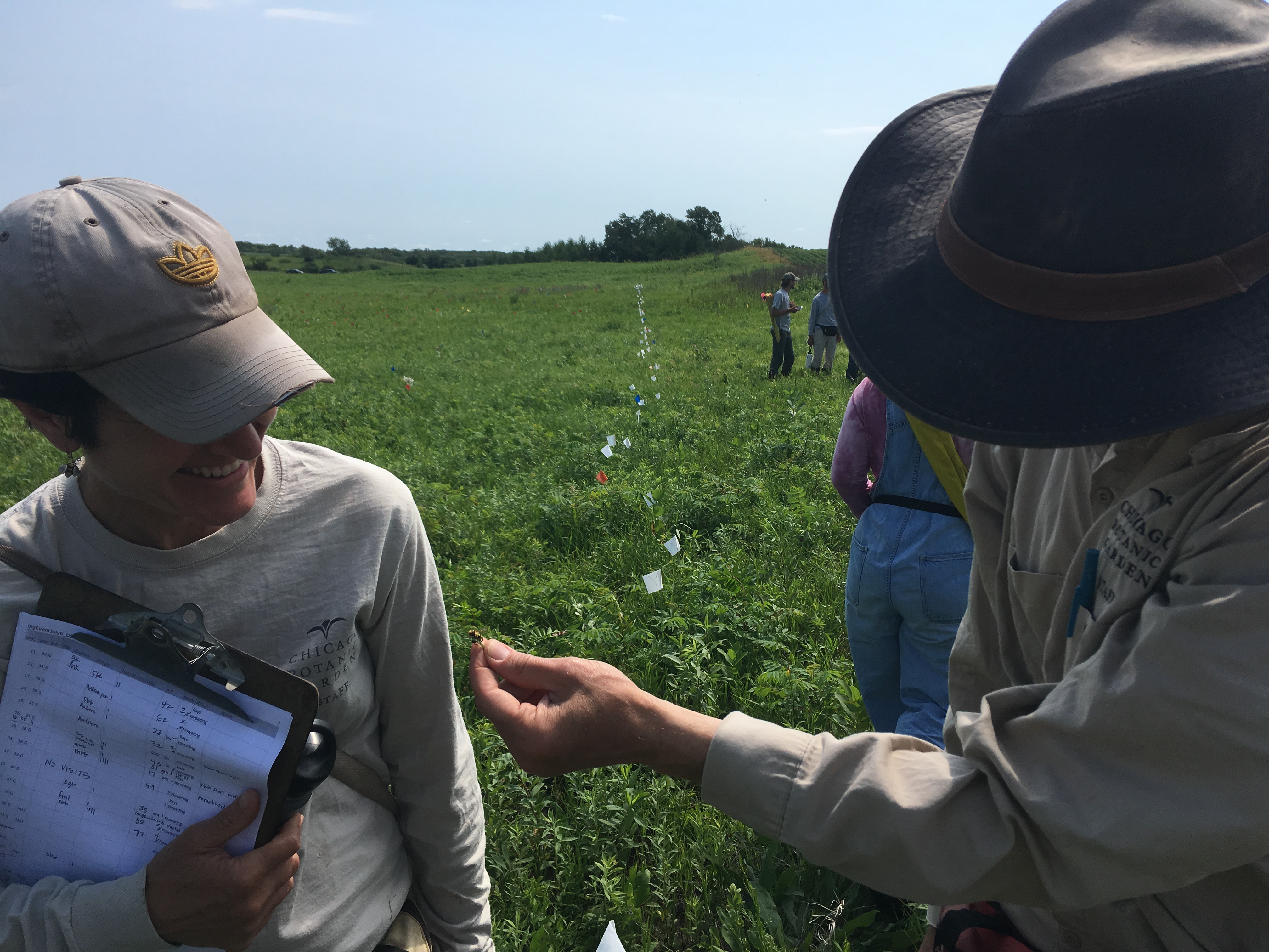
Yup you read right, today we shooed the bees from the Echinacea. Now you may be asking why would a group of scientists trying to save native bee populations tried to stop bees from pollinating flowers. Well, it’s a reasonable question. Since plants can’t move, it is difficult for them to find a mate, therefore, they have evolved to use bees to do the moving part for them. The different types of bees can have differing effects on the plant’s fitness (not how big its muscles are but how many offspring it has) and those effects are exactly what we are trying to determine with this experiment. Many plants have both male and female parts. Female being how many seeds are being made and male being how many seeds a plant helps make. This raises the question of: how good are different types of bees at distributing pollen from a plant? In order to do this, we need to have plants that are only pollinated by one type of bee. Once we have plants only pollinated by one type of bee we can track where this pollen goes using genetic work. This is where the shooing comes in, to have plants only pollinated by one type of bee we needed to shoo away the other types.
So today the entire team (except Kristen – she was busy working with bees 🙁 ) went out to P2 and worked on the male fitness project. This shooing event has been dubbed the “Big Event.” Today was the first Big Event of five(?) to come, and it was quite successful. We observed around 200 pollinators, the majority of the bees that we saw fit into the category of “small black bee” not to be confused with “medium black bees”, we also saw a fair number of Andrena which are impressive due to the great amount of pollen that each bee carries.
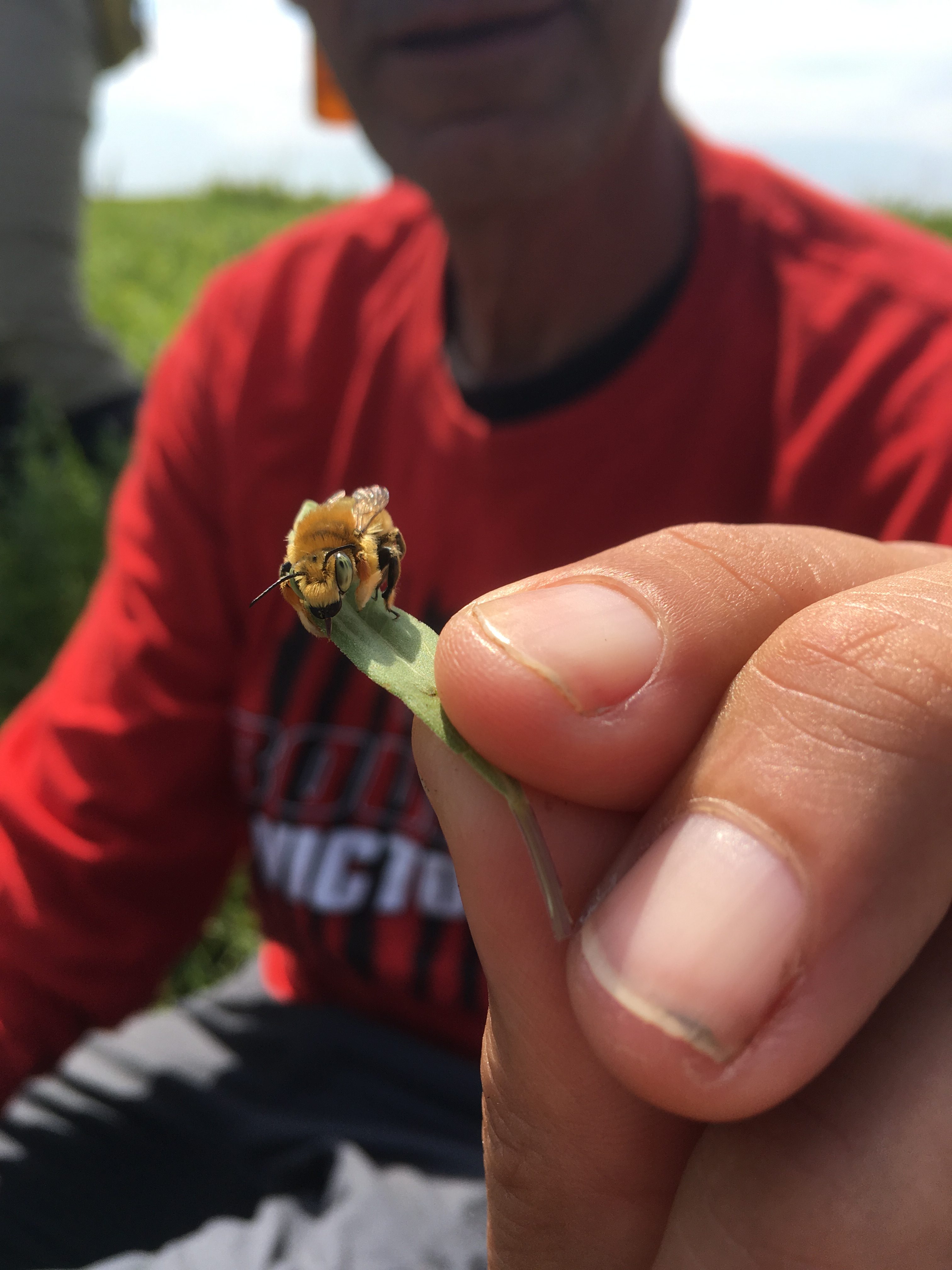
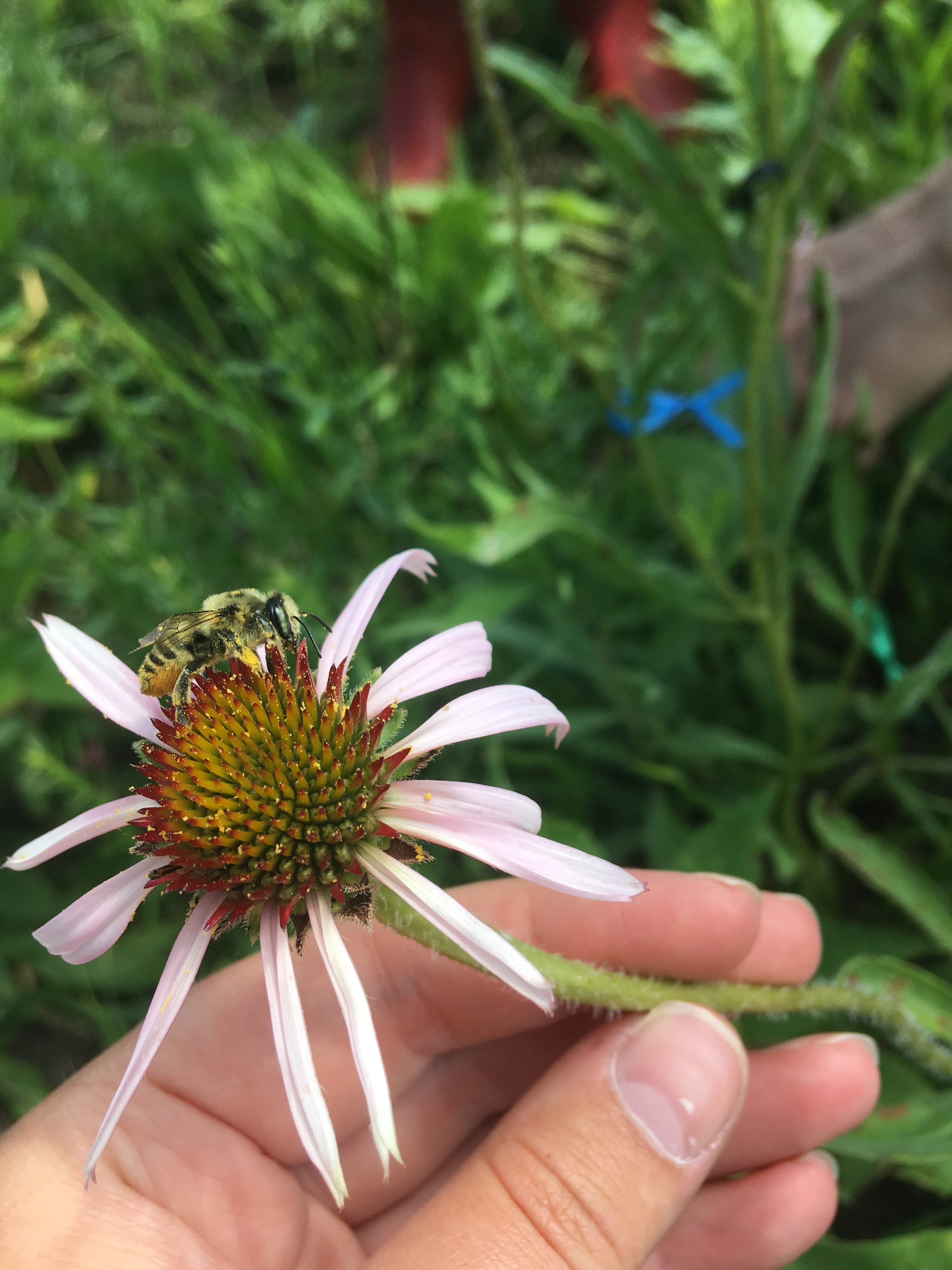
John holding a male Megachile
We saw some Augochlorellas, and Agapostomons – both of which are neat because they are green! My favorite of the day was a male Megachile which I have never seen before. They are very distinct with hairs on their front legs. This mere two and half hours of observations show you the high level of diversity of different bee species at one of our study sites! Can’t wait for the next Big Event titled Big Event 2: Electric Boogaloo and all of the bees that will be found then!
Gretel and Stuart examining a bee
A female Megachile on a echinacea(notice how she caries pollen on her abdomen)
This year, the number of flowering plants in our main experimental plot (exPt1) dropped in half compared to last year. This might be due to the lack of a burn in the prior fall or spring. Plot 2 (exPt2) had about the same number of heads in ’16 & ’17.
In exPt1, we kept track of approximately 72 heads. The peak date was July 19th. The first head started flowering on July 2nd and the last head finished up on August 21st. In contrast, we kept track of 1076 heads in exPt2, about 140 more than last year! The peak date for these Echinacea was a bit earlier, July 13th. exPt2 heads also started and ended earlier (June 22 – August 19).
We harvested the heads at the end of the field season and brought them back to the lab, where we will count fruits (achenes) and assess seed set.
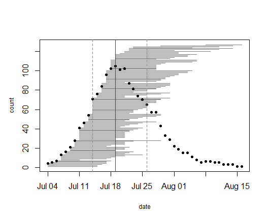
Flowering schedules for 2017 in exPt1 and exPt2. Black dots indicate the number of flowering heads on each date. Gray horizontal line segments represent the duration of each head’s flowering and are ordered by start date. The solid vertical line indicates peak flowering, while the dashed lines indicate the dates when 25% and 75% of heads had begun flowering, respectively. Note the difference in y-axes between the two plots. Click to enlarge!
Physical specimens: Harvested heads from both experimental plots are in the lab at CBG. The ACE protocol for these heads will begin soon.
Data collected: We visit all plants with flowering heads every 2-3 days starting before they flower until they are done flowering to record start and end dates of flowering for all heads. We managed phenology data in R and added it to our long-term dataset. The figures above were generated using package mateable in R. If you want to make figures like this one, download package mateable from CRAN!
You can find more information about phenology in experimental plots and links to previous flog posts regarding this experiment at the background page for the experiment.
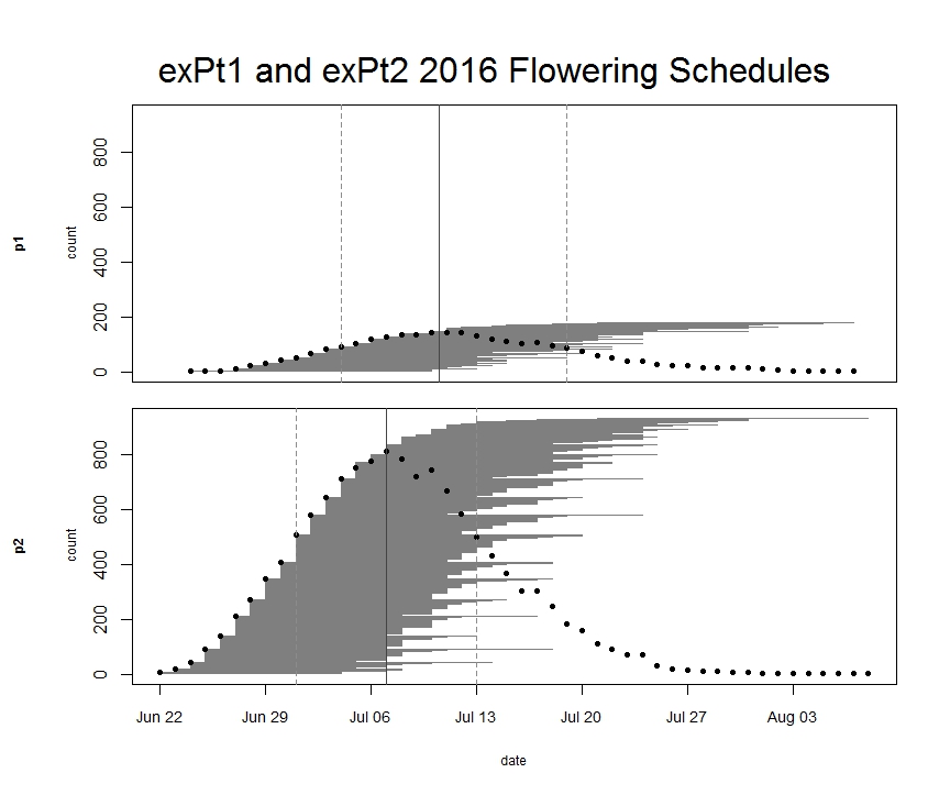
Every year we keep track of flowering phenology in our main experimental plots, exPt1 and exPt2. Fewer plants than usual flowered in exPt1 in 2016: 149 plants (179 heads) flowered between June 24th and August 7th. The population’s mean start date of flowering was July 5th and the mean end date was July 18th. Peak flowering in 2016 was on July 10th, when 143 heads were in flower. For comparison, peak flowering in 2015 was on July 27th, when there were nearly 10x as many heads flowering as on this year’s peak. The earlier phenology and low numbers of flowering we observed this year relative to 2015 is likely due at least in part to the plot burn schedule (2015 was a burn year and 2016 was a non-burn year), but there were still many fewer flowering plants than any season, burn or non-burn, in the past 10 years.
We kept track of 934 flowering heads in ExPt2, where the first head started shedding pollen on June 22 and the latest bloomer ended flowering on August 8th. Peak flowering was on July 7th, when 810 heads were flowering. ExPt2 was designed to study the heritability of phenology—you can read more about progress of that experiment in the upcoming 2016 heritability of phenology project status update.
At the end of the season we harvested the heads and brought them back to the lab, where we will count fruits (achenes) and assess seed set.
ExPt1 and Expt2 flowering schedules from 2016. Dots represent the number of flowering heads on each date. Horizontal line segments represent the duration of each heads flowering and are ordered by start date. The solid vertical line indicates peak flowering, while the dashed lines indicate the dates when 25% and 75% of heads had begun flowering, respectively. Click to enlarge!
Physical specimens: We harvested 177 heads from exPt1 and 870 from exPt2. Attentive readers may note that we harvested about 64 fewer heads than we tracked for phenology. That’s because before we could harvest many seedheads at exPt2, rodents chewed through their stems and ate some fruits (achenes). We recovered most of the heads that were grazed from the ground and made estimates of number of fruits lost due to herbivory, but we couldn’t find some heads. Arg. We brought the harvest back to the lab, where we will count fruits and assess seed set.
Data collected: We visit all plants with flowering heads every three days until they are done flowering to record start and end dates of flowering for all heads. We managed phenology data in R and added it to the full dataset. The figure above was generated using package mateable in R. If you want to make figures like this one, download package mateable from CRAN!
You can find more information about phenology in experimental plots and links to previous flog posts regarding this experiment at the background page for the experiment.
Description: In 2008 Caroline Ridley established an experiment to investigate next generation effects of genetic rescue on plant fitness. We are comparing fitness (recruitment and survival) of seeds collected from plants in the INB1 experiment in exPt 1. All of the maternal plants in INB1 were open-pollinated and in one of three groups: 1. individuals with parents from a single large remnant population, 2. individuals with parents from a small remnant population (non-rescued), and 3. individuals with parents from a large and small remnant (rescued). Eri and NWLF served as “small” remnant populations, while Lf and SPP were the “large” remnants. Rescued individuals were offspring of crosses using Eri × SPP, Eri × Lf, NWLF × SPP and NWLF × Lf.
Caroline sowed achenes in an experimental plot at Hegg Lake WMA. The plot (exPt 4) has 3 blocks, each with 2 rows. Sets of achenes (East & West) were sowed in 50-cm segments within the rows. Caroline searched for and marked seedlings with colored toothpicks in May 2009. Team Echinacea assessed late season survival in August 2009. Since then we have annually assessed survival and growth of these plants. When an individual flowers we will measure reproductive fitness!
Flowering of Echinacea angustifolia in almost all prairie remnants was down this year. Overall, approximately half as many plants flowered this year as last. Two areas distinctly bucked the trend: flowering was high at Hegg Lake WMA, which was burned this spring, and at our main experimental plot, which was burned this spring. Burning really encourages flowering!
We finished our first round of mapping all flowering plants in nearby remnants and a summary of the raw dataset is shown below. Each line lists the name of a site and the count of demo records and survey records at the site–also the difference in counts. We call our visits to remnants to find and refind plants “demography,” or demo for short. We call mapping the plants surveying because we used to use a survey station. Now we use a survey-grade RTK GPS (a Topcon GRS-1).
Notice that most sites have more demo records than survey records. This is because each data recorder enters an empty record at the beginning and end of demoing a site. Also, in certain circumstances we do demo on non-flowering plants.
Something strange is going on with the on27 site. I think someone may have entered the incorrect site name when doing demo. Also, lf looks strange, but is easily explained: lf is divided into two hills (lfe and lfw). We distinguished the two when doing demo, but not when surveying. Our next field activity is to verify the demo and survey dataset and make sure everything makes sense. Being people, we sometimes make mistakes in data entry. Because we know we make mistakes, we generate two separate datasets of flowering records (demo and surv) and compare them. When records don’t match, we go back and check.
We assess survival and reproduction of Echinacea plants in remnants to understand the population dynamics of these remnant populations. We want to know if the populations are growing, holding their own, or shrinking. To figure this out will take a few years because plants live a long time. Estimating a population’s growth trajectory based on just a couple of years of flowering records probably won’t be that informative.