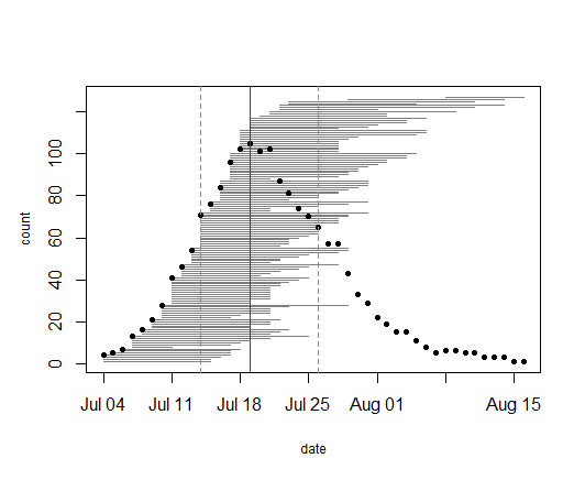
In 2019,
we collected data on the timing of flowering for 95 flowering plants (127
flowering heads) in 8 remnant populations, which ranged from 1 to 29 flowering heads.
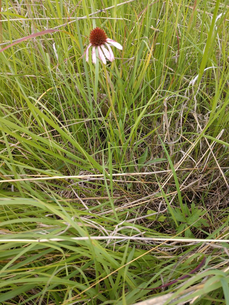
The earliest bloomers (four plants at four different remnants) initiated
flowering on July 4. Plant 24050 in the aptly named remnant population North of
Northwest of Landfill was the latest bloomer, shedding its last anthers of
pollen on August 16. Township mowers had mowed over this plant earlier in the
season, which is perhaps why it took longer for it to sprout a new flowering
stem. Altogether, the flowering season was 43 days long. Peak flowering was on
July 19, when 105 heads were flowering.
This season
marked the 19th season of collecting phenology records in remnant populations! Though
we do not have data for all populations every year, Stuart monitored phenology
in all of our remnant populations in 1996 and in following years (2007, 2009,
2011-2019) students and interns studied phenology in particular populations. From
2014-2016, determining flowering phenology was a major focus of the summer
fieldwork, with Team Echinacea tracking phenology in all plants in all of our
remnant populations. The motivation behind this study is to understand how
timing of flowering affects the mating patterns and fitness of individuals in
natural populations.
Flowering
occurred much later this season than previous years, with peak flowering
falling a full 14 days later in the year than 2018, when flowering started on
June 20, and 10 days later than 2017. Of all the years that we data for flowering
phenology in the remnant populations in and around Solem Township, this season was
the second-latest, with only the 2013 season beginning later, on July 6.
However, this observation comes with the caveat that sampling effort varied
between years and some years focused on particular contexts, such as population
where a portion had experienced a spring burn (see Fire and Flowering at SPP). Many other plants and animals in
Minnesota seemed to have delayed phenology this spring and summer, perhaps a
result of an unusually wet and snowy spring.
Start
year: 1996
Location: Roadsides,
railroad rights of way, and nature preserves in and around Solem Township, MN
Overlaps
with: phenology in experimental plots, demography in the
remnants, gene flow in remnants, reproductive fitness in remnants
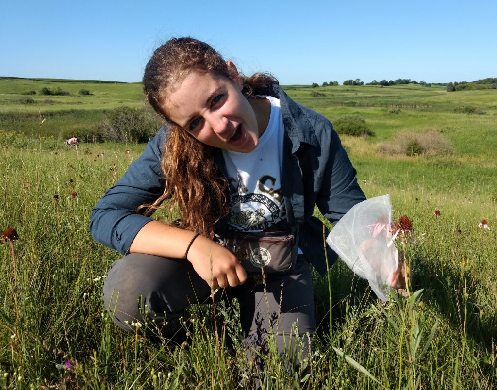
Data/materials
collected:We identify each plant with a numbered tag affixed to
the base and give each head a colored twist tie, so that each head has a unique
tag/twist-tie combination, or “head ID”, under which we store all phenology
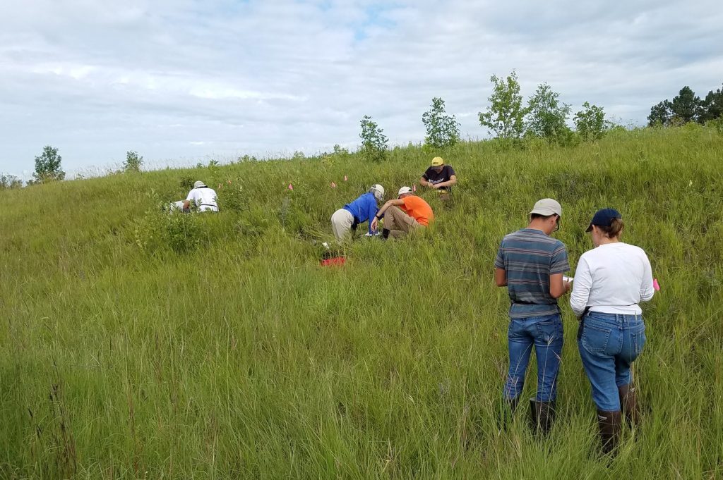
data.We monitor the flowering status of all flowering plants in
the remnants, visiting at least once every three days (usually every two days)
until all heads were done flowering to obtain start and end dates of flowering.
We managed the data in the R project ‘aiisummer2019′ and added the records to
the database of previous years’ remnant phenology records, which is located
here: https://echinaceaproject.org/datasets/remnant-phen/.
A flowering curve (created here using the R package mateable) summarizes the flowering phenology data that we collected in 2019, indicating the number of individuals flowering on a given day and the flowering period for all individuals over the course of the season.
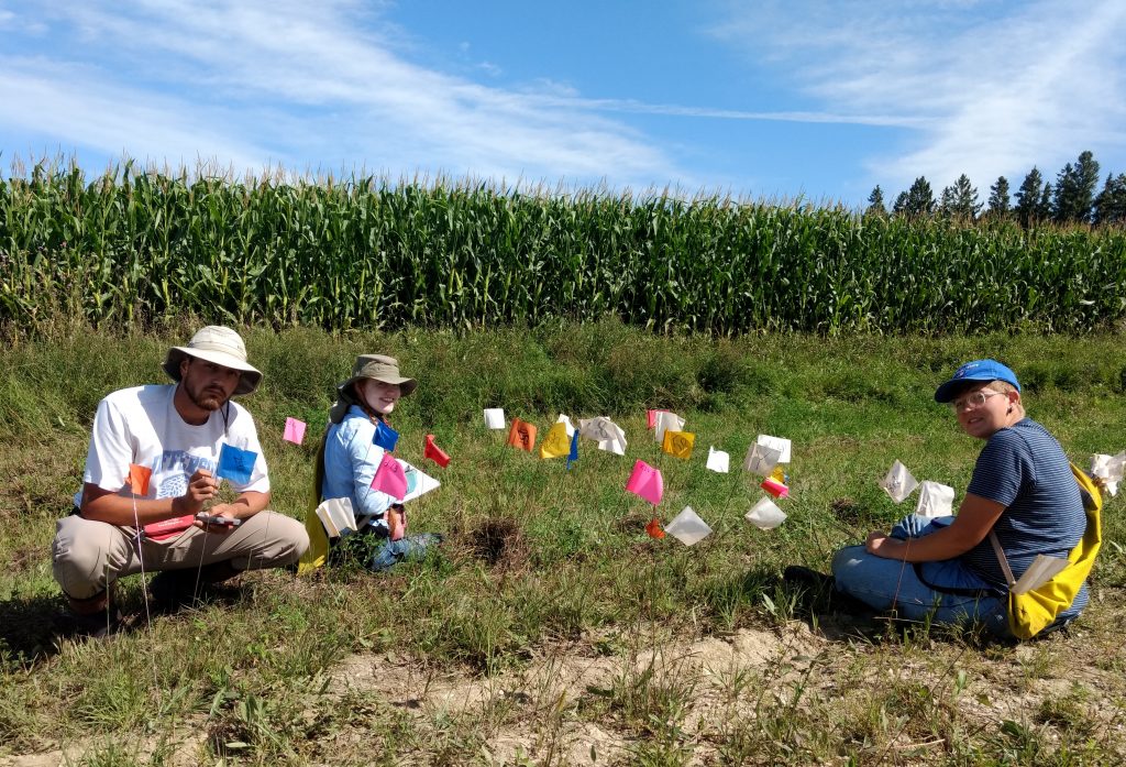
We shot
GPS points at all of the plants we monitored. Soon, we will align the locations
of plants this year with previously recorded locations and given a unique
identifier (‘AKA’). We will link this year’s phenology and survey records via
the headID to AKA table.
We
harvested a random sample of 1/3 of the flowering heads from each remnants in
August and September, plus an X additional heads from populations that were highly
isolated, for a total of X harvested seedheads. These are currently stored at
the University of Minnesota. This winter, I will assess the relationship
between phenology and reproductive fitness by x-raying all of the seeds we collected.
In addition, I will determine the paternity (i.e., pollen source) for a sample
of seeds by matching the seed genotype to the potential pollen donors. Doing so
will shed light on how phenology influences pollen movement and gene flow
patterns.
You can
find more information about phenology in the remnants and links to previous
flog posts regarding this experiment at the background
page for the experiment.
Products: I presented a poster based on the
locations and flowering phenology of individuals from summer 2018 at the
International Pollinator Conference in Davis, CA this summer. The poster is
linked here: https://echinaceaproject.org/international-pollinator-conference/.
Small remnant Echinacea populations may suffer from
inbreeding depression. To assess whether gene flow (in the form of pollen) from
another population could “rescue” these populations from inbreeding depression,
we hand pollinated Echinacea from six different prairie remnants with pollen
from a large prairie remnant (Staffanson Prairie) and from a relatively small
population that we call “Northwest Landfill.” We also performed
within-population crosses as a control. Amy Dykstra planted achenes (seeds)
that resulted from these crosses in an experimental plot at Hegg Lake WMA.
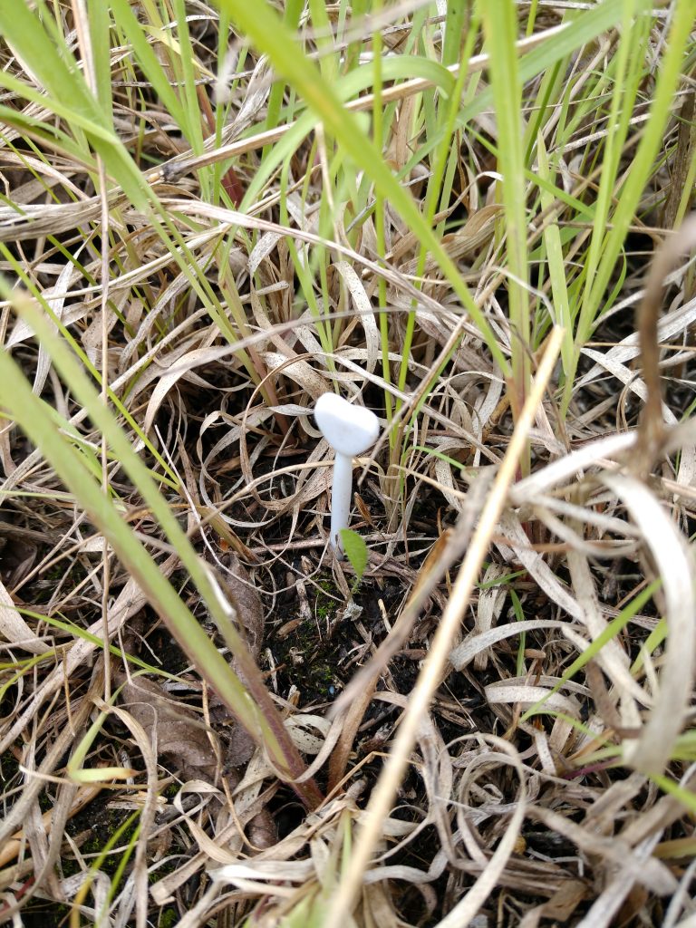
Plants in the crossing plots were originally found as seedlings like this one
We sowed a total of 15,491 achenes in 2008. 449 of these
achenes germinated and emerged as seedlings. Each summer we census the
surviving plants and measure them. This summer we found 48 surviving plants.
None of these plants has flowered, but we think some of them are close! The
largest plant we measured had 4 leaves, the longest of which was 35 cm.
You can read more about the interpopulation crosses, as well as links to prior flog entries mentioning the experiment, on the background page for this experiment.
Start year: 2008
Location: Hegg
Lake WMA
Data collected: Plant
fitness measurements (plant status, number of rosettes, number of leaves, and
length of longest leaf), and notes about herbivory. Contact Amy Dykstra to
access this data.
Products: Dykstra, A. B. 2013. Seedling recruitment in fragmented populations of Echinacea angustifolia. Ph.D. Dissertation. University of Minnesota. PDF
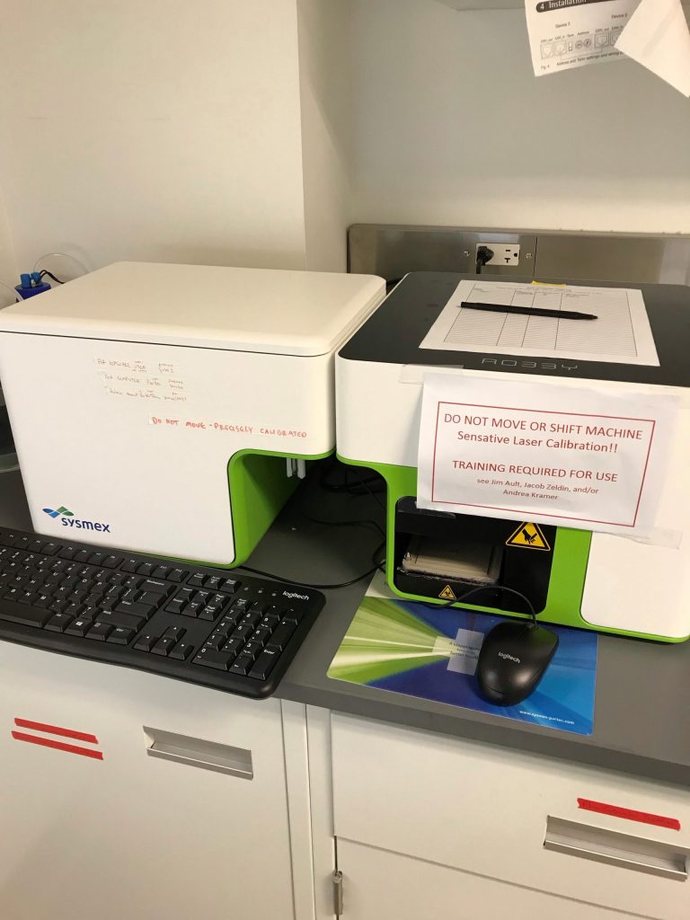
To see how ploidy varies in Echinacea species in our study site, in fall 2019, wecollected and dried tissue from E. pallida, E. angustifolia, and E. purpurea. We also collected tissue from potential hybrids and known hybrids. We brought the dried tissue back to the Chicago Botanic Garden, where we plan to analyze ploidy using a flow cytometer, a device that can be used to find relative genome size.
The flow cytometer used to assess relative genome size. Although it just looks like a box, it is truly a powerful machine.
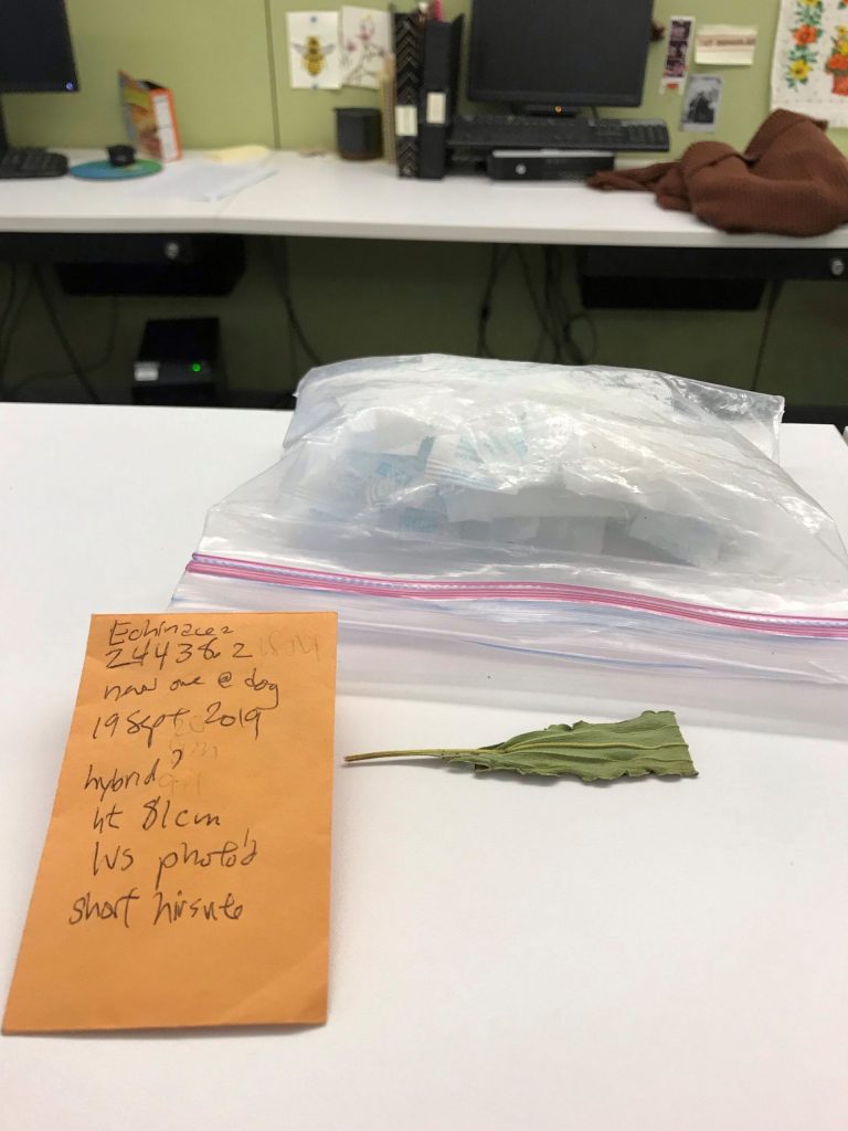
Example of dried Echinacea tissue… We thought it might be a hybrid when we visited it in the field!
Unfortunately, preparing samples for the flow cytometer is difficult, so we are going to first optimize our Echinacea tissue preparation protocol using live tissue. To do this, we withdrew accessions of E. angustifolia, E. pallida, and E. purpurea from Millennium Seed Bank at the CBG. For E. pallida, we took seed from collections throughout its range to see if its ploidy varies with latitude. We are currently germinating this live tissue to use for ploidy analysis with Elif. We are very excited to see what we find – any finding will help expand genomic knowledge for the genus Echinacea!
Start year: 2019
Location: Hegg Lake WMA, various prairie remnants and
restorations, hybrid experimental plots
Data/ materials collected:Dried tissue from
plants throughout the study area; samples are currently held at Chicago Botanic
Garden, in a small box in the glass cupboard to the right upon entering room 159,
the Population Biology Lab. Updates will be posted when genome data is
available.
In 2019 Team Echinacea conducted a new experiment called
“Pulse-Steady,” with roots in Ashley Barto’s 2017 REU project. The experiment investigates
whether flowering Echinacea plants which received a resource pulse (pollination
every three days) set seed at a different rate to Echinacea which received a
steady flow of resources (pollination every day.)
Shea expresses frustration with the bees who beat us to the pollen—bagging flowering plants to ensure we had pollen sources became critical at the end of flowering!
Stuart and Gretel selected 48 flowering Echinacea with
single flowering heads and assigned 24 to the pulse treatment, and the other 24
to the steady treatment. The team placed pollinator exclusion bags on the heads
of all plants prior to the beginning of flowering to ensure that humans were
the only pollinators. The team returned to exPt 2 every day from July 16 to
August 7 to count anthers and styles and hand-pollinate the 48 heads, though
rain caused pollen to present at strange times or not at all on some days. The
team collected pollen from other flowering plants in exPt2 as well as bagged
heads around Hegg Lake. Pollen samples included a minimum of four sires to
ensure that compatible S-alleles were present in the mix. Pollinators collected
additional pollen from heads in the experiment after pollinating the styles, to
prevent self-pollen from clogging the styles and to replenish dwindling pollen
supplies. Human pollinators frequently competed with insect pollinators, as
pollen was scarce at the end of the flowering season, and had to wave off bees
from taking pollen from experimental heads and pollen donors in the plot.
In December, Carleton externs Jack, Eli and Emma worked on a
modified ACE protocol to process the harvested pulse-steady heads. They cleaned
the heads and carefully separated the achenes based on their position in the
head so that we can investigate whether seed set differs at the beginning,
middle and end of flowering between the treatments, as well as whether seed set
differs based on style “freshness” in the pulse treatment. They also scanned
the heads with achenes separated out by location in the head.
Data/materials collected: The team harvested 48 heads in the experiment which have been cleaned and are ready to be randomized and x-rayed at the CBG. Each head has 8 envelopes associated with it (7 envelopes of achenes and 1 of chaff.)
Maps and datasheets for the field experiment are located at
~Dropbox\teamEchinacea2019\pulseSteady
The cleaning protocol and datasheets relevant to cleaning
are located at ~Dropbox\CGData\150_clean\clean2019\inb2PulseSteady
This experiment was designed to study how well adapted Echinacea populations are to their local environments. Amy collected achenes from Echinacea populations in western South Dakota, central South Dakota, and Minnesota, and then sowed seeds from all three sources into experimental plots near each collection site. You can read more about the experiment and see a map of the seed source sites on the background page for this experiment.
This summer, during our annual census of the experimental plots, we found 67 living Echinacea plants in the western South Dakota plot, including 9 flowering plants. We found 116 living plants, including one flowering plant in the Minnesota plot. This was the first flowering plant in the Minnesota plot! (We abandoned the central SD plot after it was inadvertently sprayed in 2009, killing all the Echinacea). For more details and graphs, please read this brief report.
First flowering plant in the MN local adaptation plot!
Start year: 2008
Location: Grand River National Grassland (Western South
Dakota), Samuel H. Ordway Prairie (Central South Dakota), Staffanson Prairie
Preserve (West Central Minnesota), and Hegg Lake WMA (West Central Minnesota).
Data/ materials collected: Plant fitness measurements
(plant status, number of rosettes, number of leaves, and length of longest
leaf), heads from all flowering plants
Products: Dykstra,
A. B. 2013. Seedling recruitment in fragmented populations of Echinacea angustifolia. Ph.D.
Dissertation. University of Minnesota. PDF
This past week, I continued work on multiple projects. I continued to recheck and label cleaned Echinacea heads, growing the supply of achenes that are ready to be scanned, so that we can keep the samples moving through the steps. I also spent considerable time on randomizing. I resorted the informative and uninformative achenes from some of the 2013 and 2014 collection so that they are organized in the same way as more recent samples and so protocol is consistent across the board. After resorting was complete, I did the standard randomization protocol on achenes from 2018.
In addition to working with the Echinacea collection, I continued to organized the native bee collection. One task in particular has been going through the specimens, checking the SPID numbers, and checking them off on a data sheet to confirm which specimens still exist in the collection and which ones have been removed or discarded. I have labeled each smaller box within the cases with Roman numerals and have recorded on the data sheet in which box each specimen can be found. I will continue this project in the last few days of my internship and hopefully complete it so that there is a definite record of the specimens in the native bee collection.
This field season the team continued the seedling
recruitment experiment begun in 2007. The original goal of the project was to
determine the rates of establishment and growth of seedlings in remnant
populations of Echinacea angustifolia.
From 2007 to 2013, plants which had flowered in the preceding year were visited
in the spring to find any resulting seedlings. Each fall since then the team
visits the plants, re-finds the seedlings and measures the living offspring.
In 2019 Team Echinacea visited 69 focal maternal plants in
12 prairie remnants to determine the survival and growth of their offspring.
The team searched for 128 of the original 955 seedlings and found 87 of them
(10 fewer than were found in 2018.) However, the team also re-found 27 seedlings
which could not be located in 2018. None of the original seedlings flowered
this year.
In addition to the annual seedling search, in 2019 the team
began working on a project to relate the fitness and mating scene of maternal
plants to their offspring. In late October 2019, Erin and Riley staked to the
locations of 451 maternal plants included in the original experiment which now
have “inactive” circles with no living seedlings. They visited these maternal
plants because they were not included in demo in 2018 or 2019, and their goal
was to determine the status of every original maternal plant. Since then, a
group of Team Echinacea alums and current members has begun working to prepare
the data for analysis in 2020 with the goal of submitting a manuscript in the
spring.
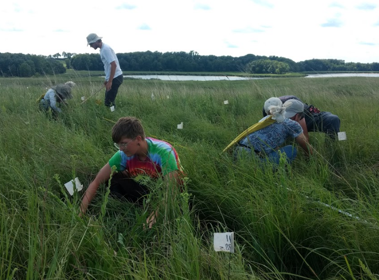
The first day of searching occurred at East Elk Lake Road, where 13 of the original maternal plants still have living offspring.
Sites with seedling searches East Elk Lake Road, East Riley, East of Town Hall, KJ’s, Loeffler’s Corner, Landfill, Nessman, Northwest of Landfill, Riley, Steven’s Approach, South of Golf Course, Staffanson Prairie
Data/materials collected: The EchinaceaSeedlings repository holds the data for this experiment. Lea Richardson restructured the repo in December 2019 to facilitate collaboration on the new project.
Notes on the project and master datasheet scans are at ~Dropbox\remData\115_trackSeedlings\slingRefindsFall2019
Data specific to the new 2019 project, including maps and
datasheets used to refind the inactive circle maternal plants, is at ~Dropbox\slingProject2019
Team members involved
with the 2019 project: Lea Richardson, Erin Eichenberger, Riley Thoen,
Drake Mullett, Amy Waananen, Scott Nordstrom, Will Reed, Amy Dykstra, Gretel
Kiefer , Stuart Wagenius
Products: Amy Dykstra used seedling survival data from 2010 and 2011 to model population growth rates as a part of her dissertation.
You can read more about seedling establishment, as well as links to prior flog entries mentioning the experiment, on the background page for this experiment.
Poor weather conditions delayed demo this year but did not
dampen our spirits! In 2019 Team Echinacea added 4031 visor records to demo and
1431 GPS points to surv. The largest effort this summer occurred at Aanenson
where eight team members took demo records on over 200 flowering plants. We
found flowering plants at Northwest of Landfill with tags from 1995 in situ, meaning the plants were at
least several years older than most of the team. We also found non-angustifolia
Echinacea invading prairie remnants Dog and Yellow Orchid Hill.
The team does demo at everyone’s favorite site: East Riley! Also known as Whose Loc Is It Anyway? Where the status is “Can’t find” and the GPS points don’t matter.
This year we performed demo and surv at 32 prairie remnants
and 10 additional sites with angustifolia populations. For our smaller sites we
visit every mature plant (ones which have flowered before.) At the larger sites
we measure a subsample of the mature population. At every site we also perform
flowering demo, where we visit plants which flowered for the first time or were
not included in the subsample. We record the status of each plant we visit, its
neighbors and the number of heads it produced. All flowering plants are tagged
and shot in surv, and in the coming months we will use demap to reconcile the
2019 demo and surv records with each other as well as those from previous years
to construct our spatial dataset of reproductive fitness in the tallgrass
prairies of our study area.
Total Demo Bill Thom’s Gate, Common Garden, Dog, East of Town Hall, Golf Course, Hegg Lake, Martinson’s Approach, Nessman, North of Golf Course, REL, RHE, RHP, RHS, RHX, RKE, RKW, Randt, Railroad Crossing Douglas County, South of Golf Course, Sign, Town Hall, Tower, Transplant Plot, West of Aanenson, Woody’s, Yellow Orchid Hill
Annual Sample Aanenson, Around Landfill, East Elk Lake Road, East Riley, KJ’s, Krusmark’s , Loeffler’s Corner, Landfill, North of Railroad Crossing, Norwest of Landfill and North of Northwest of Landfill (lumped,) On 27, Riley, Railroad Crossing, Steven’s Approach, Staffanson Prairie
In addition to the annual collection of data, this year Erin
began developing a study to investigate whether flowering return interval and
isolation by distance are correlated in Echinacea.
Start year: 1995
Location: Unbroken (never tilled) remnant prairies in Douglas County, MN, located along roadsides, nature preserves, railroad right-of-ways and privately-owned land.
Data: Access the most recent copies of allDemoDemo.RData and allSurv.RData at ~Dropbox\demapSupplements\demapInputFiles. Demap accepts these files and the demap team will clean and reconcile them in the demap repository. ~Dropbox\geospatialDataBackup2019 houses the raw GPS jobs while the aiisummer2019 repo houses the raw demo records.
Data related to
the flowering isolation study can be found in the floiso repository (contact
Erin Eichenberger for access) and in the folder ~Dropbox\floweringIsolation2019
Products: Amy Dykstra’s dissertation included matrix projection modeling using demographic data
Project “demap” merges phenological, spatial and demographic data for remnant plants
You can read more about the demographic census in the remnants, as well as links to prior flog entries mentioning the experiment, on the background page for this experiment.
Since 1996, members of Team Echinacea have walked, crawled, and ~sometimes~ run next to rows of Echinacea angustifolia planted in common garden experiments. Although protocol varies depending on the common garden, every year team members record flowering phenology data, measuring data, and harvest the heads of the thousands of plants we have in common garden experiments. The Echinacea Project currently has 10 established experimental plots: exPts1-10. Due to the repetitiveness of yearly phenology, measuring, and harvesting, this project status report will include updates on all common garden experiments except for Amy Dykstra’s plot (exPt3), qgen2qgen3 (exPt8), and the West Central Area common garden (exPt10).
exPt1: Experimental plot 1 was first planted in 1996 (cleverly termed the 1996 cohort), and has been planted numerous times in subsequent years, with the most recent planting being inbreeding 2. It is the largest of the experimental plots, with over 10,000 planted positions; experiments in the plot include testing fitness differences between remnants (1996, 1997, 1999) effects of inbreeding (inb1, inb2), and quantitative genetics experiments (qgen1). There are also a number of smaller experiments in it, including fitness of Hesperostipa spartea, aphid addition/exclusion, and pollen addition/exclusion. In 2019, we visited 4392 of the original 10,622 planted and found 3486 alive. Only 70 plants were classified as “flowering” in exPt1 this year. This is a drastic change from the nearly 1000 plants that flowered in summer 2018 – perhaps it is a testament to the benefits of controlled burning (we burned in spring 2018 but not in 2019). In summer 2019, we harvested 52 total Echinacea heads in exPt1. In the fall, we added 789 staples to positions where plants were gone for three straight years – this was desperately needed because no staples were added to positions with dead plants after 2018.
exPt2: Heritability of flowering time is the name of the game in exPt2. Planted in 2006, exPt2 was planted to assess if flowering start date and duration was heritable in Echinacea. In summer 2019, we visited 2050 positions of the 3961 positions originally planted. We measured 1802 living plants, of which 654 were flowering. In the fall, we harvested ~1100 heads from exPt2. We do not have an exact number of heads harvested from exPt2 yet, as we have not had time to complete head reconciliation. Location: Hegg Lake WMA
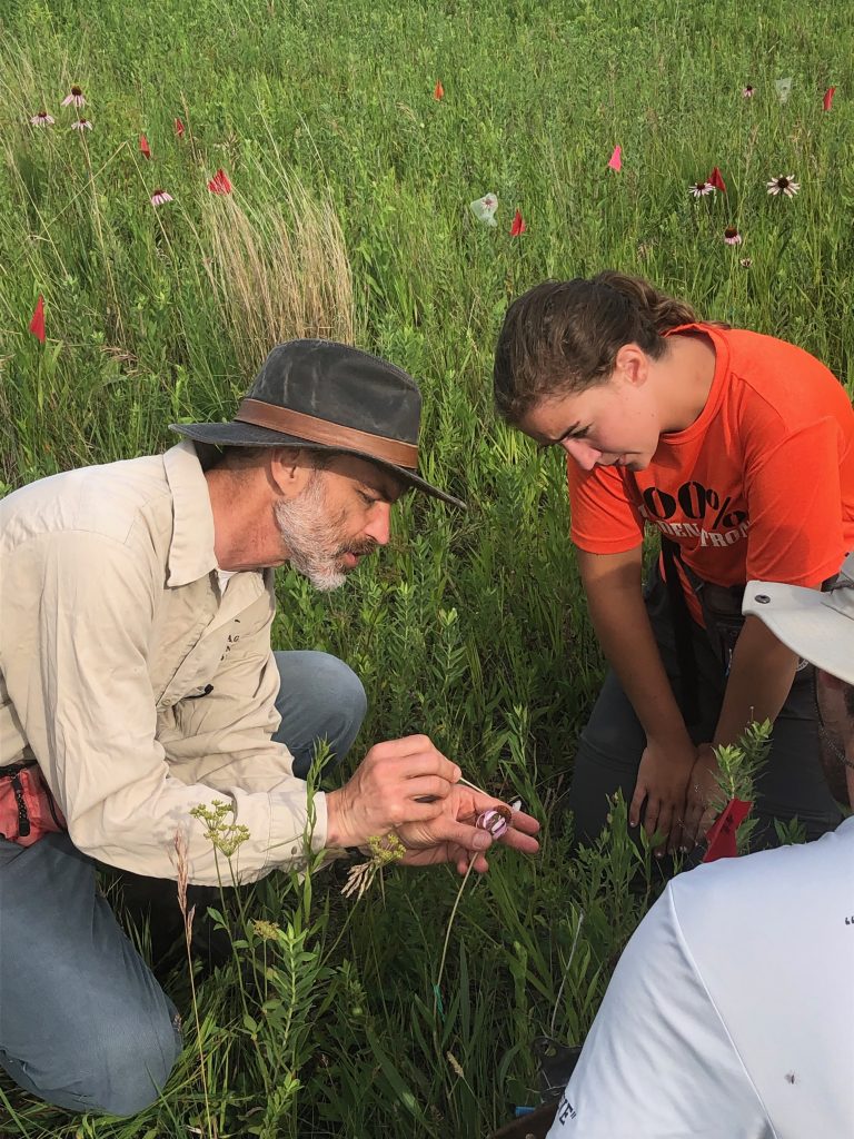
Stuart explains Echinacea capitulum morphology to Shea in one of the experimental plots.
exPt4: Experimental plot 4 was planted to determine if Echinacea from small remnant populations could be genetically rescued via an outcross to larger, more genetically diverse populations. Caroline Ridley and other members of Team Echinacea sowed 3584 achenes at Hegg Lake WMA in 2008, and we have assessed survival and basal plant characters every year since. Survival in exPt4 is incredibly low. We only visited 21 plants in 2019 and only 7 were alive. No plants have flowered in this plot yet. Location: Hegg Lake WMA
exPt5: The only experimental plot planted at Staffanson Prairie Preserve (SPP), exPt5, was planted in an attempt to compare progeny of maternal plants from burned and unburned sections of SPP. There were 2800 plants planted originally, but high mortality made it impossible to visit the plot row-by-row. Now, we and treat the plot like demography. We use a GPS to find plants in exPt5 that have previously flowered and add more plants to the stake file if new plants in the plot flower. In 2019, we visited 10 plants in the plot, all of which were alive! There were no plants flowering in exPt5 in 2019, though. Location: Staffanson Prairie Preserve
exPt6: Experimental plot 6 was the first E. angustifolia x E. pallida hybrid plot planted by Team Echinacea. A total of 66 Echinacea hybrids were originally planted; all have E. angustifolia dams and E. pallida sires. In 2019, we visited 40 positions and found 28 living plants. No plants have flowered in this plot yet. As of January 2020, all exPt6 measure data through summer 2019 is uploaded to the SQL database. Location: near exPt8
exPt7: Planted in 2013, experimental plot 7 was the second E. pallida x E. angustifolia plot. It contains conspecific crosses of each species as well as reciprocal hybrids. There were 294 plants planted. Out of the 205 plants we visited in 2019, we found 161 plants still alive and basal; there were no flowering plants this year. For some context, survival of pure E. angustifolia crosses was lower than all other cross types. As of January 2020, all exPt7 measure data through summer 2019 is uploaded to the SQL database. Location: Hegg Lake WMA
exPt9: Experimental plot 9 is another hybrid plot, but unlike the other two hybrid plots, we do not have a perfect pedigree of the plants. That is because E. angustifolia and E. pallida maternal plants used to generate seedlings for exPt9 were open-pollinated. We need to do paternity analysis to find the true hybrid nature of these crosses (assuming there are any hybrids). There were originally 745 seedlings planted in exPt9, and in 2019 we visited 510 positions. It was one of the harder plots to measure because over half of the positions did not have a plant and we do not use staples at Hegg Lake WMA. We found 308 living plants in 2019, one of which was flowering! We know the flowering plant has an E. pallida mother, but we are still unsure of the paternity of the flowering plant. When we know, we will post an update. As of January 2020, all exPt9 measure data through summer 2019 is uploaded to the SQL database. Location: Hegg Lake WMA
Summer 2019 measures exPt9… so many “Can’t Finds!”
For more information on survival in common garden experiments, see this flog post about survival in common gardens.
Start year: Various, see individual listings above. First ever
planting was 1996.
Location: Various, see above
Overlaps with: Pretty much everything we do
Data/ materials collected:Measure data for
all plots. All raw measure data available in cgData repository. Processed data should
eventually be available in SQL database; ask GK for status of SQL database. GPS
points were shot for the exPt9 flowering plant, as well as for all surviving
plants in exPt4. Find the GPS jobs containing the exPt4 and exPt9 points in
~Dropbox\geospatialDataBackup2019, saved in three formats in
temporaryDarwBackups2019, convertedXML2019 and convertedASVandCSV2019. The job
name is SURV_20191002_DARW and the points have names that distinguish them by
the experimental plot. The stake file to find exPt5 plants is here: ~Dropbox\geospatialDataBackup2019\stakeFiles2019\exPtFiles\exPt05stakeFile.csv
Products: Many publications and independent projects.
This summer Jay Fordham conducted an experiment in
experimental plot 8 to determine an effective method for eradicating Fraxinus pennsylvanica, or green ash.
Team Echinacea is concerned with the spread of green ash in our experimental
plots because it crowds out native herbs. The Echinacea in exPt8 may be at
particular risk due to their young age relative to individuals in other plots.
A prior attempt to manage ash in exPt8 with triclopyr (brand name Garlon)
largely failed, resulting in only 3% mortality.
Jay devised three treatments of triclopyr application to green ash. The three treatments were 1) A foliar application where he painted all leaves with triclopyr; 2) A bark application where he cut each ash 10cm from the base and applied triclopyr to the remaining above-ground stem; and 3) A cambium application where he cut each ash 10cm from the base, scraped off the exterior bark with a knife, and applied triclopyr to the remaining above-ground stem. He divided exPt8 into 35 treatment sections and randomly assigned a treatment to each section. He then randomized the treatment application order and, with the help of the team, treated 438 green ash trees from July 22nd to August 8th. Jay then assessed ash mortality on August 27th and 28th and found the cambium application to be most effective. Jay presented his findings at the 2019 Midstates Undergraduate Research Symposium in St. Louis on November 1-2. His presentation is available to view and download here.
Triclopyr treatment
Mean Proportion Dead Stems
Foliar application
0.005
Cutting and bark application
0.333
Cutting and cambium application
0.498
In addition to the green ash management experiment in exPt8,
the team removed Bird’s-foot trefoil from exPt1 and along the bordering road.
The team also removed sweet clover from within and around exPt1, exPt2 and
exPt3. The team cut back sumac from the easternmost rows of exPt1.
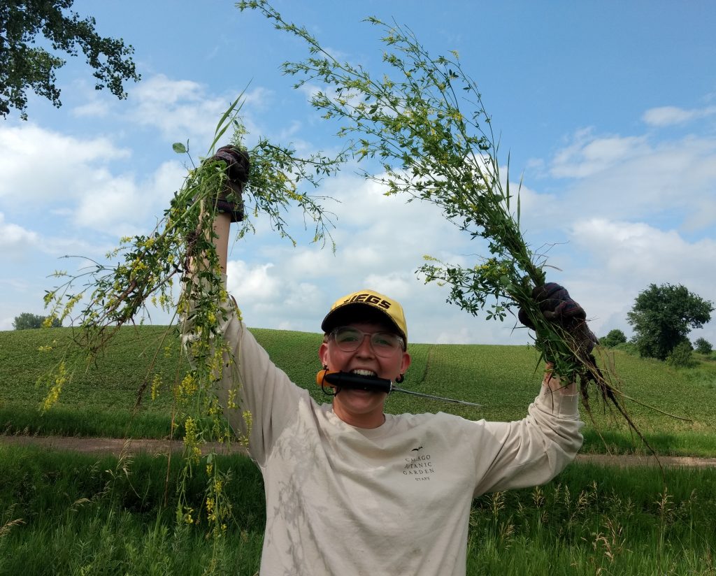
Jay brandishing sweet clover plants that the team pulled in exPt1
In June the team planted Asclepias
viridiflora in exPt1 at regular intervals. Stuart initially assessed
approximately 124 surviving plugs prior to planting. Erin and Riley, while
pulling flags marking the planting locations in September, did not observe any
surviving milkweed plants. The team also planted Carex gravida and Carex
brevior in the path around exPt1. The team planted three of the same carex
species at each location in a triangular configuration. Erin shot the planting
positions with the GPS pole in the center of the three plants, or between two
where two survived, or north of a single plant where one survived. In October
she observed that approximately 2/3rds of the carex plantings were present.
Location: exPts 1, 2 and 8
Data/materials collected: Weeds were discarded outside the plot as they were removed.
Find information about Jay’s experiment at
~Dropbox\teamEchinacea2019\jayFordham
Find information about the planting locations of the
Asclepias viridiflora at ~Dropbox\CGData\Asclepias\plantPlugs2019.csv
Find the two GPS jobs containing the carex locations in
~Dropbox\geospatialDataBackup2019, saved in three formats in
temporaryDarwBackups2019, convertedXML2019 and convertedASVandCSV2019. The job
names are CAREX_P1_20190801_DARW and CAREX_P1_20191003_DARW.