Trevor Hughes

Prof. Wagenius

8 December 2017

Field Site Burning Effects on Liatris and Solidago Species: Year 2

Background Info:

       Habitat fragmentation threatens the livelihood of many remnant prairie populations in the midwestern United States. This is the result of various biological mechanisms such as limited genetic diversity and transformation of the surrounding ecosystem, both of which yield direct effects on the plant species coexisting there (Newman and Pilson 1997, Saccheri et al. 1998). Through either modification potential mates location as well as other changes in pollinator behavior, the reproduction of these species is left especially vulnerable to change (Wagenius 2006). These reproduction patterns are measured in what is commonly referred to as seedset, or the percentage of fertile achenes (those that possess an embryo) out of a certain grouping of total achenes; therefore, seedset effectively displays the relative amount of achenes that are fertile on any given inflorescence.

       Previous research reveals that both pollinator activity and respective reproduction of native plant species decrease with habitat fragmentation; as well, many of these studies focused on select species, namely the Echinacea angustifolia, a common plant species often found in midwestern prairie remnant habitats (Wagenius 2006). Differing from prior research, this study focuses on how a contemporary trend—the burning of a specific remnant prairie habitat—could be affecting the reproductive activity of remnant prairie plant species. Expanding beyond Echinacea, this study focuses on two other key prairie species: Liatris and Solidago. By examining two different sides (east and west) of a specific remnant prairie site where the east and west sides are burned interchangeably on a repeating pattern: east side burned, west side burned, and no side is burned. This report analyzes the findings concerning the second year of the study, where no field site was burned. While the specific findings discussed will be limited to this year’s data, with next years data, the study hopes to aggregate all years to yield some conclusions as to the effects of field site burning on reproduction of prairie plant species. Aside from investigating the possible effect that field-site burning has on the seedset of the plant species in the area, it also hopes to be able to provide comparable findings between Liatris, Solidago, and Echinacea so that findings regarding habitat fragmentation can be generalized to more prairie plant species in the future.

Methods:

       Liatris and Solidago were gathered at the Staffanson site within the Douglas county in western Minnesota (centered near 45°49’ N, 95°43’ W). They were collected using a randomized method, with 90 Liatris and 74 Solidago inflorescences collected in total. However, the Liatris and Solidago species were collected from both the East and West sides of the Staffanson site, but a blind-procedure was used to ensure this was not known during the data collection or analysis process. It should be noted that while the West field site was burned last year, no field site was burned this year in preparation for burning the East field site and continuing the cycle in 2018.

       Following the collection process, the Liatris and Solidago inflorescences were randomized using excel software and put in their appropriate order, divided by species. This prevents bias at multiple steps during the course of data collection, including cleaning, counting, and x-raying. Beginning with Liatris, a bag was selected according to the random order and all heads were removed from the inflorescence to be cleaned. Next, thirty achenes were selected randomly using a grid system under the container to be used as an x-ray sample for that inflorescence. The remaining achenes were separated from any chaff and placed in an envelope for future reference and potential research. This process was repeated with all 90 Liatris samples. Additionally, beginning with the 50th randomized Liatris sample and continuing until all remaining Liatris samples were cleaned, the number of achenes in the top, middle, and bottom head were also recorded in a spreadsheet. If there was no clear middle, the achene closest to the bottom relative to the midpoint was chosen.

       The Solidago process was quite similar. The bags were selected in a pre-randomized order and the inflorescence was removed to be cleaned. However, due to the considerable number of achenes on most Solidago inflorescence, it would be impractical to attempt to use all achenes for cleaning; therefore, I simply shook each inflorescence for 10 seconds and used those achenes for further analysis. From there, 30 achenes were randomly placed into a small plastic baggie for x-raying whilst other achenes were separated and placed into an envelope for further comparison. This process was repeated for all 74 solidago samples.

       After the cleaning was completed, the baggies were placed on sheets to prepare for x-raying. Twenty samples were x-rayed at a time and there scans were recorded. Lastly, the x-ray samples were counted for the number the number of achenes in each sample that actually contained a fertile embryo; in this way, the seed-set of the Liatris and Solidago achenes was recorded so that comparisons between the east and west Staffanson field sites could be made.

Results:

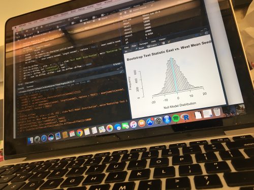
       All data was aggregated and analyzed with use of various statistical tests on the R platform; all figures and/or tables were also made on this same platform. Data regarding the top/middle/bottom breakdown of Liatris along with the seedset of Liatris and Solidago on the east and west sides of the Staffanson site were analyzed for potential findings.

Figure 1: Location of Head vs. Size of Head in Tops/Middles/Bottoms of Liatris

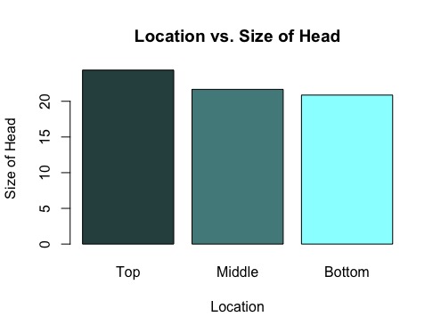
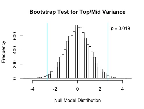
       The tops of the Liatris species were found to have the greatest number of achenes with a mean number of achenes of 24.367, middles followed with a mean of 21.667, and bottoms yielded the lowest mean at 20.867 (see Figure 1). A bootstrap test was conducted between the means of the tops and middles, generating a p-value of 0.019, meaning that there is only a 1.9% chance that the difference in size of head betweenst tops and middles would be found by chance simply by sampling randomly from inflorescences (see Figure 2). While a p-value was not calculated for the difference in size of head amongst tops and bottoms, it is speculated that this analysis would yield a even lower p-value than tops and middles due to the greater difference in mean. While a bootstrap test was run between middles and bottoms,  this yielded a high p-value and indicated there was a large possibility that the difference between middles and bottoms of Liaris could be found by chance from sampling randomly and was therefore not determined to be an meaningful finding.

Figure 2: Bootstrap Test for variance between Tops and Middles of Liatris

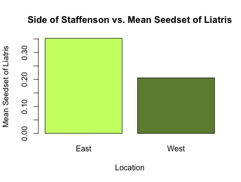
       The data collected on seedset for the 90 Liatris samples was aggregated and eventually divided between East and West lines of the Staffanson site. The mean seedset was calculated for each side and are compared below (see Figure 3). The East meen seedset of Liatris was 35.2%, which towers over the West’s 20.6%.

Figure 3: Side of Staffanson Site vs. Mean Seedset of Liatris

       A bootstrap test was run on this dichotomy to determine the confidence intervals of these findings as well as the p-value. The ablines were found to fall outside of the normal distribution, yielding a p-value of 0.1%, indicating that this difference has a very little possibility of resulting from chance and that the difference in seedset between the East and West is quite noteworthy and telling of other possible differences between these two sites. The confidence intervals were not found to overlap, strengthening the certainty of my findings (see Figure 4).

Figure 4: East and West Sides of Staffanson vs. Mean Seedset of Liatris with 95% C.I.

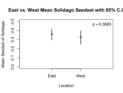
       Identical tests were conducted on the 74 Solidago samples and respective seedset data, but different findings were discovered. The seed-set data collected for Solidago was divided between the east and west sides of the Staffanson site. The mean seed-sets of each side were calculated, revealing to be 35.9% for the east and 32.7% for the west (see Figure 5). This demonstrates that the east had a higher seed-set, but not at the same large interval seen with the Liatris species. Confidence intervals and a p-value were also determined for each side. The p-value was revealed to be 36.45%, which indicates the potential for this difference in seed-set to result a large portion of the time from natural variation, and not possibly due to the difference in side of the Staffanson site (see Figure 6). Supporting this large p-value, the confidence intervals also overlap, indicating that the variables could potentially swap and vary greatly in repeating this study, generating further doubt on the implications of this finding.

Figure 5: Side of Staffanson Site vs. Mean Seedset of Solidago

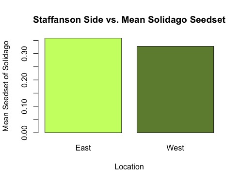
Figure 6: East and West Sides of Staffanson vs. Mean Seedset of Solidago with 95% C.I.

Discussion:

Firstly, the data regarding the tops/middles/bottoms of Liatris demonstrate a definite correlation among location and size of head. Based on the low p-value, it can be determined that the tops have the greatest number of achenes, compared to the middles and bottoms, but whether or not there is a significant difference in the number of achenes betweenst middles and bottoms cannot be directly determined from this data set. While this data indicates a trend between location and size of head (with greatest numbers of achenes found among the top heads), more samples should be collected and  analyzed to strengthen this finding, specifically with regards to the difference in size between middles and bottoms.

Before the data from this years seedset among the east and west sides of the Staffanson site can be analyzed, the findings from last year’s study (when the West side was burned), must be discussed. The 2016 data indicates that the West had a higher mean seedset than the East for Liatris, but there was little to no correlation between the east and west with Solidago. This finding is interesting for a couple of reasons. For one, this directly contrasts with my data from this year (where no sides were burned), as now the east had nearly a 75% increase in seedset compared to the West. Interestingly, the east side now has the larger seedset, meaning the sides of the field swapped by a large margin. This also contrasts with what one would expect with a field burning, which generally is speculated to stimulate growth, achene development, and seedset. However, it appears from this data set that the burning possibly hinders achene development and seedset, but this cannot be completely determined from this data set. The data from 2018 (when the East side is burned), would be vital for drawing this conclusion.

Interestingly enough, while the data sets contradict themselves on these grounds, they agree on one important point: field site burnings have a greater impact on Liatris than Solidago. This raises questions as to what biological mechanism within each species accounts for this difference. Once again, data from 2018 would also be vital for making a definitive conclusion as to why field site burning seems to have a lessened impact on the Solidago species.

Nina here! Today was Trevor and I’s last day of our externship, which was bittersweet. Although I’m very excited to sleep in past 6:30, I’m definitely going to miss our mentors, Tracy, Lea, and Stuart, as well as all of the volunteers and the whole Botanic Garden community that we briefly got to know during our time here. Trevor and I mostly continued working on our papers, but we also gave short presentations of our projects to the lab to practice presenting. We also had closing interviews regarding our experiences and our thoughts on the externship. Trevor and I have both really enjoyed our time with the Echinacea project, and we hope that you will stay tuned for our final papers, which will be coming very soon (either this weekend or on Monday).

Thanks for everything,

Nina 🙂

Nina here! Today, Trevor and I continued analyzing the data that we collected during the first two weeks of our externship. We both kept working in R, perfecting our papers, and analyzing our results.

Trevor found the confidence intervals for mean seed-set for Liatris and was very excited to see that the two intervals didn’t overlap, strengthening his confidence in his previous findings. Next, he aggregated and merged Solidago data before repeating the analysis he did for Liatris on the Solidago data, but with very different results. It seems as if Solidago was not effected by the burn that occurred in the site (as you can see from the photo on the left), but stay tuned for more updates!

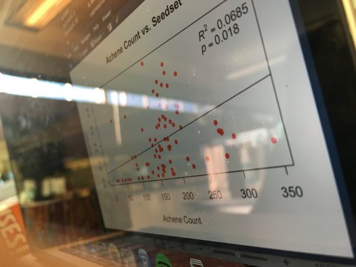Meanwhile, I looked the diversity function within R’s ‘vegan’ package to use Shannon’s and Simpson’s Diversity Indices on my plant community from each plot. I plotted seed-set, fecundity, and achene count against each index and found the highest correlation when looking at achene count. Next, I calculated species richness as well as the Shannon’s and Simpson’s Diversity Indices including only flowering plants. More updates to follow! After finishing up my actual analysis, I got back to working on my paper (which you can see a preview of on the right) and started thinking about which portions of my results and which graphs I might want to include in my paper.

Nina here! To start off the third week of our externship, Trevor and I got back to work in R. We started making our own scripts to try to visualize our data and understand our results. I found a strong correlation between seed-set and fecundity and a correlation between seed-set and achene count (although the R squared value was small). I downloaded a database of plants of Minnesota from the USDA database that included information on whether or not the plants were native, threatened, or endangered as well as their fire tolerance and growth habit. I merged this database with the diversity data collected in the field in order to provide more data about each species. Next, I tried to calculate the percent of invasive and nonnative species for each plot. Meanwhile, Trevor calculated the means for the numbers of achenes in the top, middle, and bottom samples and determined whether or not there was statistical significance between pairwise comparisons of the findings. Next, he looked at confidence intervals for his findings. We both continued our work on our papers, writing up our methods sections specifically. As Trevor meant to say, there’s nowhere to go from here but up!

Nina here! Today, Trevor and I downloaded R and RStudio and started familiarizing ourselves with R by using the tutorial package ‘swirl’ and completing several of the lessons about the basic building blocks, vectors, matrices, data frames, logic, functions, and much more! Thanks in part to Trevor’s donut holes and Tracy and Lea’s support, we powered through and completed the swirl tutorials. Next, I got started with looking at my own data by reading in some of the csv data files into R and trying to get started on viewing them and writing a script to determine species richness. Also, just for fun, here’s a counting timelapse from a couple days ago of an evaluating empty, partially empty, and full achenes!