|
|
This summer, I’ve been working on an experiment examining style age, pollination treatment, and row position. For future members of Team Echinacea, I wanted to share my data with them. 🙂
To this post, I’ve attached two .csv files. “HeadData_081017” includes data applicable to each head as a unit, and “RowData_081017” includes data applicable to each row. I’ve also attached a .txt file titled “PlantRowShrivelData_MetaData_081017,” which gives an overview of my experiment and explains each column in my .csv files.
.csv files:
HeadData_081017
RowData_081017
.txt file:
PlantRowShrivelData_MetaData_081017
To read the .csv files, copy this script into R:
HeadData<-read.csv(url("https://echinaceaproject.org/wp-content/uploads/2017/08/HeadData_081017.csv"))
RowData<-read.csv(url("https://echinaceaproject.org/wp-content/uploads/2017/08/RowData_081017.csv"))
Have you ever had one of those days you can just feel rain coming? Yesterday was one of those days. When I stepped outside in the morning, my immediate thought was “I wonder when it will start raining?”. The sky was ominous, and pretty much by the time we arrived at the Hjelm House it was coming down.
We spent the first part of the morning updating Stuart and Gretel on our individual projects, measuring, and demo. My yellow pan trap project is going well; I have the contents of approximately 120 traps in the Hjelm House freezer right now waiting to be pinned, and I tried to use the rainy weather yesterday to make a dent in all of that. My pinning is getting faster each day, and the pinned specimens are looking better and better. Soon I will begin identifying these specimens and analyzing my data.
It amazes me, when I think about phenology, how long it used to take to complete. I was able to do the whole of the Around Landfill loop in about half an hour yesterday, a task that would have taken two people a morning to complete only a few weeks ago. It amazes me how much time has gone by this summer already.
This brings us to the pivotal event yesterday: the great coaxial cable conundrum. In short, we need a new cable for the GPS, but the brand-name replacement is far too expensive. We spent some time discussing our options, and a decision has yet to be made. More updates to come?
The afternoon brought a little more rain, which for me meant more pinning. After the rain cleared, Wes, Ashley, Anna, and I embarked to Hegg Lake to measure at the Hybrid plot there. Unfortunately, we were unable to finish the plot, having only two or three rows remaining, but I’m sure they will be finished soon.
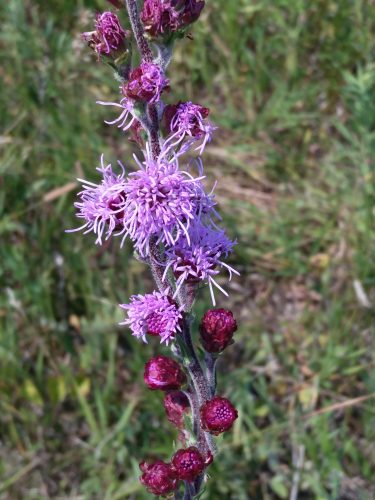
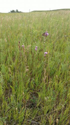
 An old image, flowering Liatris at Hegg Lake; 31? July 2017.
Today was a day full of demo. Everyone headed out to East Riley in the morning while Lea went to take data on her floral resource plots along roadsides. East Riley might not be the most exciting remnant for demo at this point in the summer, as most of the “flowering” plants we were finding were designated with an M1 or an M2 or even an M5… meaning we were just finding mowed heads that perhaps once had great potential. All of the mowing also seemed to make tons of small basal rosettes pop up, so our visor forms were reaching their max with nearby neighbors. At one point in the afternoon when we were finishing up East Riley, Lea staked around 20 plants within a .5 x .5 meter area. And there were tiny Echinacea everywhere! It was quite a puzzle.
 Anna with some high density PBORY at East Riley. Many small basal Echinacea plants and lots of locs at East Riley. Lea and I also spent some time back at Staffanson today working on our neighborhood richness vegetation project (aka RichHood). We got through 5 of our 2 x 2 meter plots today, so we are making progress! 8/100, only 92 to go! We are pretty sure our plots at Staffanson will take the longest since there is such high diversity, and therefore a lot of plants we have to spend time figuring out. It’s really fun work though.
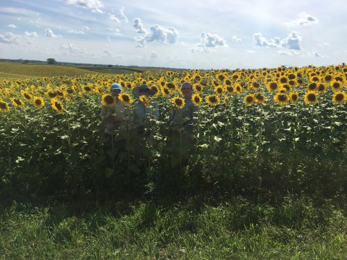
To finish off the day we did flowering demo at Yellow Orchid Hill and KJ’s, two nice roadside remnants. When we were staking the plants at Yellow Orchid Hill, the GPS went to float for a bit. However, calling on the space weather gods seemed to work quite well. In the few seconds after me calling out to them, the GPS went from Auto to Fixed! Then, we got to hang out among the sunflowers at KJ’s before heading back to the Hjelm House.
Anna, Lea, and Ashley hanging out in the sunflowers across from KJ’s! Until next time, flog!
Today was our second full day of Team Echinacea minus Stuart and Gretel. They will be back Wednesday! We managed to have a productive day anyway, though we did have less inspiring lunch conversations.
We started our morning off with a few people going on quick phenology routes. The Nessman and Around Landfill loops and p2 take less than an hour now, and I went to Staffanson just to visit 2 plants! One of those plants is now done flowering, and we’re just left with a single mid-flowering head among the ash trees. I will admit, all of these done flowering Echinacea can make me a little sad, BUT there are still plenty of other plants flowering…
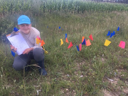
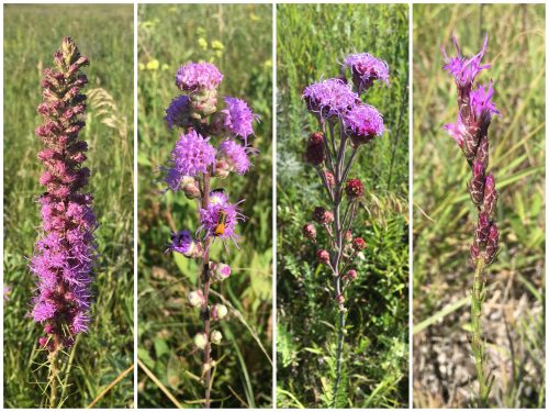
While others spent the rest of morning working on demo at East Riley or working on aphids, I helped Lea with her Liatris phenology/seed set experiment (Aster Phen). We headed out to her transect along the south part of Staffanson and finished flagging the transect, flagged Liatris aspera, and continued taking phenology data. This usually involved just counting the heads that might potentially flower and then identifying the position of the topmost flowering head and the lowermost flowering head. Most of them were still in their immature stage, just starting to get tinges of pink on the white buds. Liatris is a beautiful plant, so I will share a few of the many photos I took today while getting very excited.
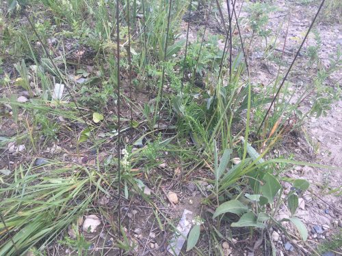
There are four species of Liatris at Staffanson. Lea studies Liatris aspera, but there are a lot of Liatris ligulistylis in and around her transect as well.
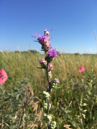
The four species of Liatris at Staffanson. From left to right: Liatris pycnostachya, Liatris aspera, Liatris ligulistylis, Liatris punctata. Collage by MOLDIV. A Liatris aspera in Lea’s transect. The Liatrus ligulistylis have lengthier branches holding the heads.
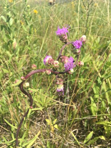
 Liatris ligulistylis with its branching heads. Some of the Liatris even get into strange shapes.
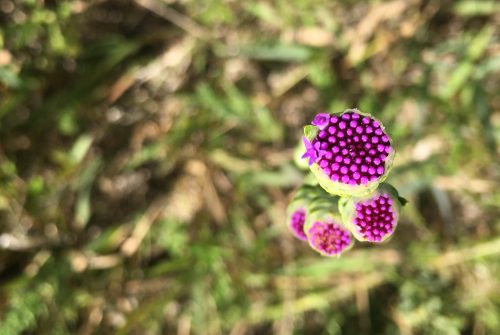
A figure-8 Liatris aspera. You can see the way the heads swirl down the stem when looking at them from above.
 A Liatris aspera with the top head barely flowering, from above. After lunch I spent more time with the Liatris and Lea before we went to help start measuring p4 and p9. Another good day.
See you tomorrow, flog!
I spent my Sunday preparing for the week and relaxing.
Lea and I went grocery shopping in the morning, and when I returned to Andes, I started Swirl in R. Between lessons, I tinkered with my pulse and steady pollination data. By Tuesday, I hope to have some basic descriptive statistics to share with the team.
So far, using the range function, I was able to see my experimental plants’ styles emerged between July 8th and July 26th, and were pollinated within the same range. I was also able to see the sum of all the styles I pollinated: 1980! Hopefully, tomorrow I can work on finding the overall average style shrivel rate on day 1 and day 2 considering both treatments, and eventually, I hope to be able to find the shrivel rate by treatment in R. While I can find these things within the spreadsheet itself, I think R is a valuable tool I can use for my data analysis for this project, and it is a skill I need to develop as a young ecologist.
Other than working in R, I enjoyed listening to the cool rain that poured over Andes, and I savored Lea’s Beaufort stew dinner. A few of us also gathered around to stream some silly shows and share a laugh.
That’s all for this relaxing and somewhat productive Sunday.
Until next time, I’ll be sharpening my R skills!
Saturday!!!! Woohoo!!!
The Andes crew took a break with many of us going in to Alexandria to do laundry, do grocery shopping, and drink coffee. I spent my late morning and afternoon out at Hegg Lake looking for candidates for seed collection. There were many flowers that were blooming, including the Rough Blazing Star (Liatris aspera).
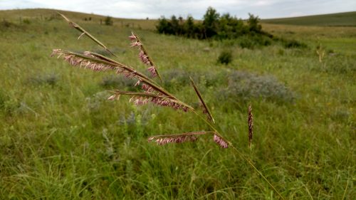
 Liatris aspera in full bloom with a monarch. A new flowering individual for me was the Prairie Cord Grass (Spartina Pectinata).
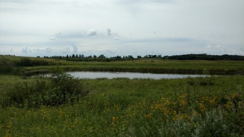
 Spartina pectinata blooming. Along with pretty plants, I had the opportunity to watch a Northern Harrier hunt and successfully catch dinner. There was also a pelican checking out a small pond.
A pelican on a pond at Hegg Lake.
What phenology means to you (in 5 words or less):
“16/10 first day, great job!”
-Wesley Braker
“Around Landfill, Monarch caterpillars”
-[possibly Anna Vold]
“one two zero one seven”
-Alexander Hajek
“Never red, white, and clear.”
-William Reed
“I’ll do the Nessman loop”
-Lea Richardson
“That’s a nice Echinacea”
-Tracie Hayes
“Let’s check the decision tree!”
-A. Barto
“This one’s not twist-tied!”
-Gretel Kiefer
“Active searching, turn your head”
-[likely Stuart]
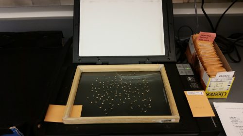
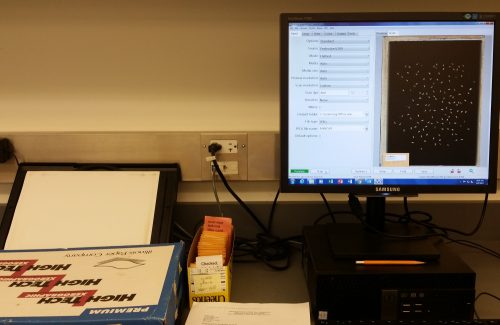
The scanned image of all the individual achenes will be used to count the number of achenes for that one head . This process allows for increased accuracy in assessing female fitness by allowing for a precise count of total achenes per head.
There is a document for the protocol of each step of scanning in addition to particular settings for the scanning software (please refer to that document for details). The document can be found in the “Protocols” folder in the lab by the light switch. First, the achenes are spread on a glass frame which is stored in the cabinet labeled “Trays for Scanning.” Spread the contents of the envelope onto the frame making sure that there are no achenes along the edge. Important to this process is that there are no overlapping achenes and that none are standing on end. Next, the envelope with the achene information should be placed at the bottom left of the glass (see image below). This whole setup is covered with a lid of a box top cover in black fabric NOT the cover that comes with the scanner.
The basic setup of scanning achenes. Double click the “VueScan” icon on the desktop to open. Make sure the settings correspond to those that are in the protocol that can be found in “Protocols” folder in the lab (once the setting is made a first time it remains but it is still a good idea to double check). The scans should be stored in a “Default Folder” on the computer; the name of the folder changes each year. The 2015 scans will be stored on the C drive in the folder entitled cg2015scans. This folder will change with the collection year. Each scan is named according to the letno on the envelope.
Once the achenes are scanned they get placed back in the envelope and any chaff or dust that may be left is put in the chaff envelope. The scanned achene envelope is then moved to the back of the box behind the marker “Scanned behind this paper.” After a box is done being scanned the envelopes of achenes and chaff move to the next step of random sampling.
 Scanned image as seen in VueScan software. Note that a box lid is used to cover the scanner bed not the original cover.
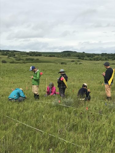
Today was a really chilly day for August. The high temperature was around 60 degrees and it rained most of last night. We did some inside work this morning while we waited for it to dry off, one team (Wes, Ashley, and Alex) went to north of railroad crossing to do total demo but, the weather did not cooperate.
This afternoon we worked on measuring plants in experimental plot 2. We began measuring in p2 midway through the morning on Tuesday. We finished measuring almost 4000 positions today. That’s only 2 days! Probably a new record measuring p2. The data we collected in p2 over the last couple days will be added to the long-term fitness data set for those plants which were planted in 2006.
We look forward to slightly warmer weather tomorrow!
Three groups diligently measure in experimental plot 2!
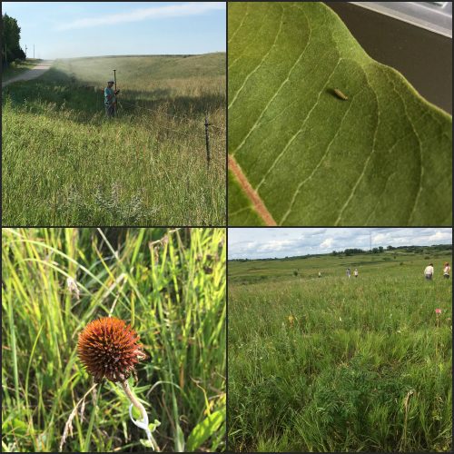
After a crazy and super fun Waterama weekend in Glenwood, it was fun to get back to work with the rest of Team Echinacea. Today was phenology Wednesday and with many of the plants done flowering it took barely an hour to complete everything! I will admit I am a little sad that summer is almost over… However, since phenology is nearing the end, we also used this morning to work on demo at north railroad crossing and around landfill. I worked with Gretel and Alex after finishing phenology at around landfill and found a tiny (hopefully monarch) caterpillar! His name is Angustus and I am hoping he will grow into a fantastic butterfly we can release soon!
After lunch, we headed out to P2 to measure. Today we got to row 37 out of 80. Even though this is less than half, the coming rows have fewer plants. When we had measured for about 3 hours, Stuart cut up a watermelon and the team enjoyed that as an end to a great day.
The plan for the rest of the week includes more demo, phenology, and other projects! Also, everyone is looking forward to the promise of a cool, 60 degree day tomorrow!
 Top left- Alex staking at alf, Angustus the caterpillar, measuring, and an Echinacea done flowering
|
|